基于 EM 算法的多元高斯混合模型聚类及其 Python 实现

基于 EM 算法，推导多元高斯混合模型聚类的参数迭代公式，并使用 Python 对数据集进行聚类和各类别的参数求解。

在编写代码的过程中，遇到了一个非常简单但一直没发现的 Bug。

定义数组用all_density = np.array([0]*K)，再用all_density[k] = k_density并不会让all_density的第k个元素改变。这是因为all_density是介于 0 到 1 之间的，而在定义all_density的时候没有指定数组内部的数据类型，默认是不支持小数的，因此赋值之后all_density的第k个元素仍然是 0。

解决方法：定义数组的时候一定要指定元素的数据类型，指定为dtype=flout64就可以存储高精度的浮点数。

问题描述

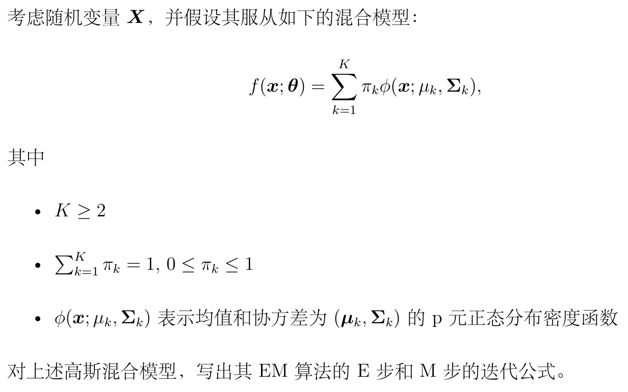
EM 算法的基本思想和具体步骤

基本思想

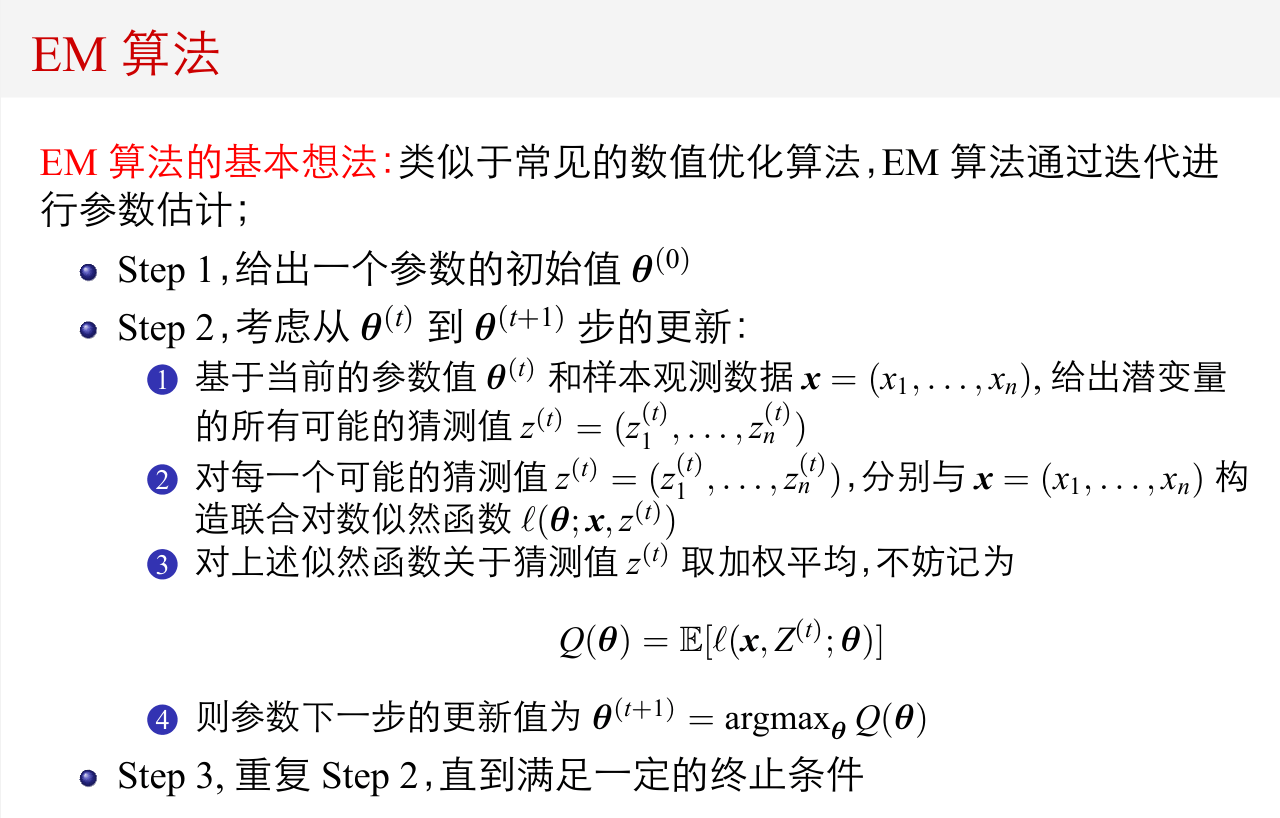
具体步骤

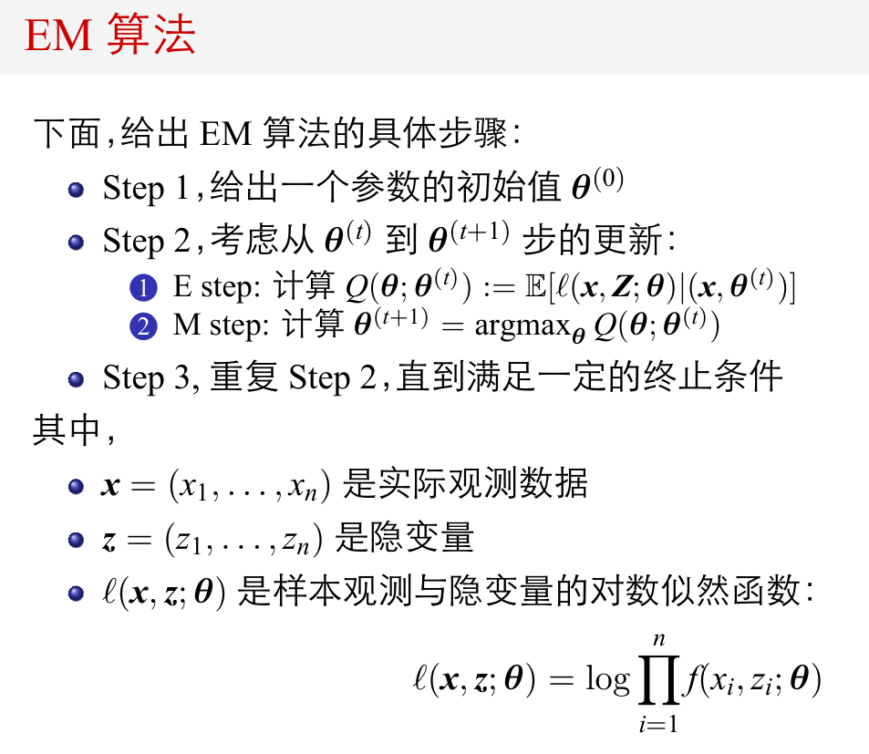
关于初始值和终止条件的几点说明

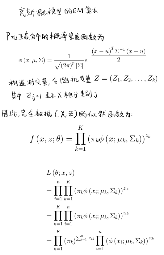
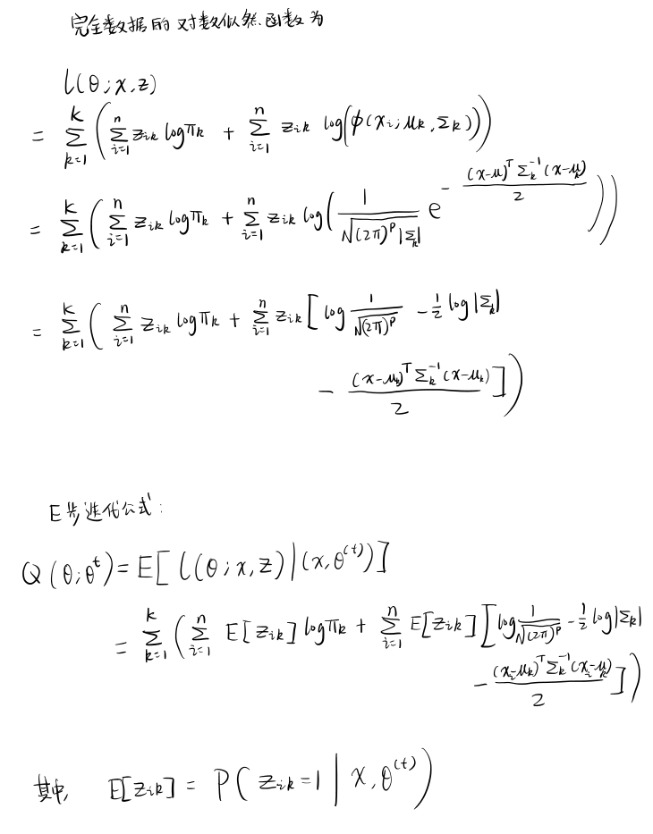
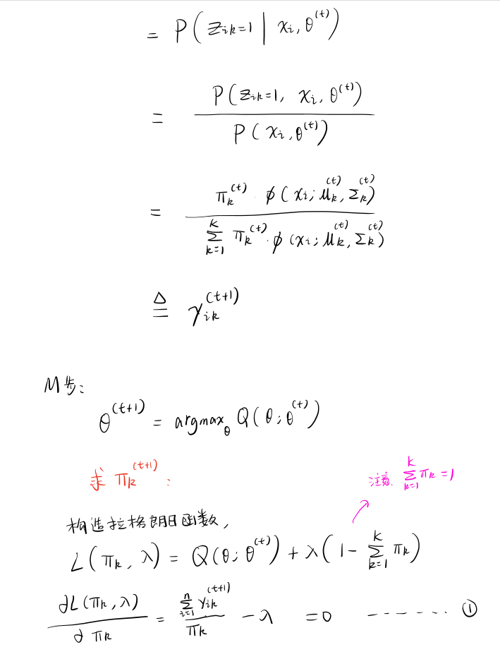
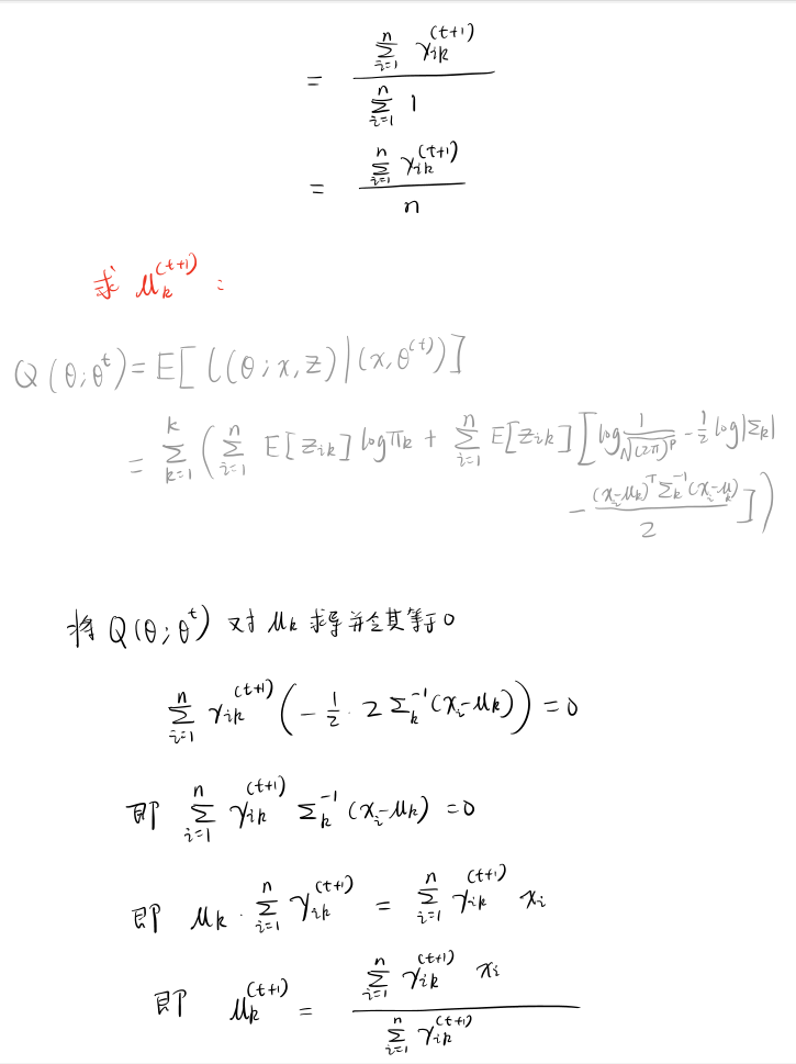
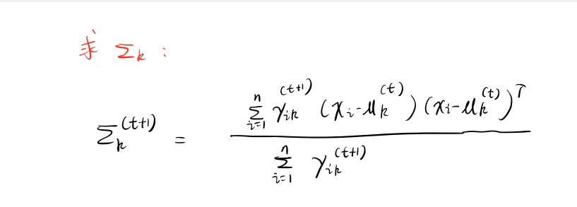
推导多元高斯混合模型聚类的参数迭代公式

使用 Python 对数据集进行聚类和各类别的参数求解

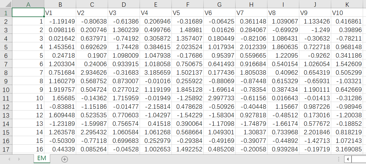
数据集描述

导入包

Python

# 导入包
import pandas as pd
import numpy as np
import matplotlib.pyplot as plt
import matplotlib.ticker as ticker

# 显示中文
plt.rcParams["font.sans-serif"] = ["SimSun"]
plt.rcParams["axes.unicode_minus"] = False
# 渲染公式
plt.rcParams["text.usetex"] = True

读取数据

Python

# 读取数据，跳过第一列
data = pd.read_csv("EM.csv", index_col=0).values
# 识别数据维度
n, p = data.shape
# 可能来自的分布数量
K = 2

给出所有参数的初始值

Python

# 初始化每个数据点来自哪个分布的概率
pai = np.array([0.5] * K, dtype=np.float64)
# 初始化均值矩阵（p*K）。一个分布的均值都是 1，另一个分布的均值都是 0
mu = np.array([[1] * p, [0] * p], dtype=np.float64).T
# 初始化协方差矩阵（p*p*K）。每个分布的协方差都是单位矩阵
sigma = np.array([np.eye(p)] * K, dtype=np.float64)
# 打印初始值
print("pai:\n{}\n\nmu:\n{}\n\nsigma:\n{}".format(pai, mu, sigma))

Text Only

## pai:
## [0.5 0.5]
##
## mu:
## [[1. 0.]
##  [1. 0.]
##  [1. 0.]
##  [1. 0.]
##  [1. 0.]
##  [1. 0.]
##  [1. 0.]
##  [1. 0.]
##  [1. 0.]
##  [1. 0.]]
##
## sigma:
## [[[1. 0. 0. 0. 0. 0. 0. 0. 0. 0.]
##   [0. 1. 0. 0. 0. 0. 0. 0. 0. 0.]
##   [0. 0. 1. 0. 0. 0. 0. 0. 0. 0.]
##   [0. 0. 0. 1. 0. 0. 0. 0. 0. 0.]
##   [0. 0. 0. 0. 1. 0. 0. 0. 0. 0.]
##   [0. 0. 0. 0. 0. 1. 0. 0. 0. 0.]
##   [0. 0. 0. 0. 0. 0. 1. 0. 0. 0.]
##   [0. 0. 0. 0. 0. 0. 0. 1. 0. 0.]
##   [0. 0. 0. 0. 0. 0. 0. 0. 1. 0.]
##   [0. 0. 0. 0. 0. 0. 0. 0. 0. 1.]]
##
##  [[1. 0. 0. 0. 0. 0. 0. 0. 0. 0.]
##   [0. 1. 0. 0. 0. 0. 0. 0. 0. 0.]
##   [0. 0. 1. 0. 0. 0. 0. 0. 0. 0.]
##   [0. 0. 0. 1. 0. 0. 0. 0. 0. 0.]
##   [0. 0. 0. 0. 1. 0. 0. 0. 0. 0.]
##   [0. 0. 0. 0. 0. 1. 0. 0. 0. 0.]
##   [0. 0. 0. 0. 0. 0. 1. 0. 0. 0.]
##   [0. 0. 0. 0. 0. 0. 0. 1. 0. 0.]
##   [0. 0. 0. 0. 0. 0. 0. 0. 1. 0.]
##   [0. 0. 0. 0. 0. 0. 0. 0. 0. 1.]]]

迭代更新参数

Python

# 求高斯分布的概率密度函数
def gaussian(x, mu, sigma):
    return (
        1
        / np.sqrt((2 * np.pi) ** p * np.linalg.det(sigma))
        * np.exp(-0.5 * (x - mu).T.dot(np.linalg.inv(sigma)).dot(x - mu))
    )


# 求给定参数下，数据点属于各分布的概率
def prob(x, mu, sigma, pai, K):
    all_density = np.array([0] * K, dtype=np.float64)
    for k in range(K):
        k_density = pai[k] * gaussian(x, mu[:, k], sigma[k])
        all_density[k] = k_density
    return all_density / all_density.sum()

Python

all_iteration_pai = [pai]
all_iteration_mu = [mu]
all_iteration_sigma = [sigma]
iteration_count = 0
while True:
    iteration_count += 1
    # 将所有样本的属于各分布的概率初始化为 0
    n_prob = np.array([[0] * K] * n, dtype=np.float64)
    # 求所有样本的属于各分布的概率
    for i in range(n):
        # 求第 i 个样本属于各分布的概率
        x = data[i, :].T
        prob_i = prob(x, mu, sigma, pai, K)
        n_prob[i] = prob_i
    # 更新 pai_k
    pai = n_prob.sum(axis=0) / n
    # 将本轮迭代的 pai 保存
    all_iteration_pai.append(pai)
    # 更新 mu
    mu = data.T.dot(n_prob) / n_prob.sum(axis=0)
    # 将本轮迭代的 mu 保存
    all_iteration_mu.append(mu)
    # 更新 sigma
    for k in range(K):
        sigma_k = np.zeros((p, p), dtype=np.float64)
        for i in range(n):
            x = data[i, :].T  # x 是列向量
            sigma_k += n_prob[i, k] * np.outer(x - mu[:, k], x - mu[:, k])
        sigma_k /= n_prob.sum(axis=0)[k]
        # sigma_k 是 10*10 的矩阵
        sigma[k] = sigma_k
    # 将本轮迭代的 sigma 保存
    all_iteration_sigma.append(sigma)
    # 判断是否达到终止 1
    new_mu = all_iteration_mu[-1]
    old_mu = all_iteration_mu[-2]
    # 当本次迭代得到的 mu 和上次迭代得到的 mu 几乎没有差别时，可以终止迭代
    if (np.subtract(new_mu, old_mu) ** 2).sum() < 1e-8:
        break

打印出迭代的次数和参数的值

Python

print("迭代次数：{}".format(iteration_count))

Text Only

## 迭代次数：17

Python

print("pai:\n{}\n".format(pai))

Text Only

## pai:
## [0.58870318 0.41129682]

Python

print("mu:\n{}\n".format(mu))

Text Only

## mu:
## [[ 1.01500407  0.18662592]
##  [ 0.97982009  0.01332565]
##  [ 1.00858025 -0.12719368]
##  [ 1.0234199  -0.02555446]
##  [ 1.04411481  0.00185229]
##  [ 1.02298727  0.00717931]
##  [ 1.01387045 -0.05989538]
##  [ 0.97264306 -0.08819002]
##  [ 0.99824314  0.22147017]
##  [ 0.92537071 -0.00442322]]

Python

print("sigma:\n{}".format(sigma))

Text Only

## sigma:
## [[[ 4.77850968e-01  2.03033657e-02  3.78546195e-02 -1.01181913e-03
##    -2.96115297e-02 -5.54141629e-03 -1.47452695e-02  1.37669547e-02
##    -6.28394728e-02 -1.21109511e-02]
##   [ 2.03033657e-02  4.77796696e-01 -6.62293811e-03  3.75985666e-02
##    -2.04491793e-02 -2.98300772e-03 -8.21489696e-03 -3.22317835e-02
##    -5.36574177e-03  4.54354716e-02]
##   [ 3.78546195e-02 -6.62293811e-03  4.54636109e-01 -3.51923568e-02
##     6.34667740e-03 -3.56763317e-02 -1.53553017e-03 -1.43510168e-02
##    -2.67175562e-02  2.75253474e-02]
##   [-1.01181913e-03  3.75985666e-02 -3.51923568e-02  4.54814674e-01
##    -1.09588387e-02 -8.04964137e-03 -6.79355591e-02 -1.58610602e-02
##     1.38411070e-03  2.97408576e-02]
##   [-2.96115297e-02 -2.04491793e-02  6.34667740e-03 -1.09588387e-02
##     4.18149094e-01  5.14822421e-02 -2.70075163e-02 -4.85719583e-02
##    -3.90824938e-02 -9.80214724e-03]
##   [-5.54141629e-03 -2.98300772e-03 -3.56763317e-02 -8.04964137e-03
##     5.14822421e-02  5.57272122e-01 -3.35251541e-03  1.08618076e-02
##    -1.70210877e-02 -3.56956117e-02]
##   [-1.47452695e-02 -8.21489696e-03 -1.53553017e-03 -6.79355591e-02
##    -2.70075163e-02 -3.35251541e-03  4.87019479e-01 -3.51035789e-02
##    -1.15753668e-02 -1.56505402e-02]
##   [ 1.37669547e-02 -3.22317835e-02 -1.43510168e-02 -1.58610602e-02
##    -4.85719583e-02  1.08618076e-02 -3.51035789e-02  4.23483429e-01
##     4.98114718e-02  2.34207606e-03]
##   [-6.28394728e-02 -5.36574177e-03 -2.67175562e-02  1.38411070e-03
##    -3.90824938e-02 -1.70210877e-02 -1.15753668e-02  4.98114718e-02
##     4.82600350e-01 -1.92214963e-02]
##   [-1.21109511e-02  4.54354716e-02  2.75253474e-02  2.97408576e-02
##    -9.80214724e-03 -3.56956117e-02 -1.56505402e-02  2.34207606e-03
##    -1.92214963e-02  5.65086238e-01]]
##
##  [[ 9.29295093e-01  4.08010510e-02 -8.23808935e-04  8.44863621e-03
##     1.20218799e-01 -1.11470574e-01  1.53808551e-02  7.88913749e-02
##    -2.78554252e-02  3.22006682e-02]
##   [ 4.08010510e-02  9.83440827e-01 -5.49377007e-02 -2.71323305e-02
##    -5.45668743e-02  1.21946570e-01  2.00130257e-02  9.74783909e-02
##    -1.53586564e-01  1.30733179e-01]
##   [-8.23808935e-04 -5.49377007e-02  1.07523742e+00  7.43292761e-02
##     3.62964590e-02 -2.81937066e-02  1.96732798e-02 -1.07758450e-01
##     8.91156366e-02 -1.92974649e-02]
##   [ 8.44863621e-03 -2.71323305e-02  7.43292761e-02  9.11091322e-01
##     1.89237737e-02 -7.29374832e-02 -1.32674621e-01 -7.57571711e-02
##     5.28107636e-02 -1.12753582e-01]
##   [ 1.20218799e-01 -5.45668743e-02  3.62964590e-02  1.89237737e-02
##     8.88748718e-01 -9.57949898e-02 -5.23966099e-02 -9.07784608e-02
##     3.94038498e-02 -7.42123835e-02]
##   [-1.11470574e-01  1.21946570e-01 -2.81937066e-02 -7.29374832e-02
##    -9.57949898e-02  1.00163225e+00  2.84507420e-02  1.29356885e-01
##     8.54158988e-02  6.04867236e-02]
##   [ 1.53808551e-02  2.00130257e-02  1.96732798e-02 -1.32674621e-01
##    -5.23966099e-02  2.84507420e-02  9.74886562e-01 -1.91740598e-02
##    -1.45956772e-01  4.74506001e-02]
##   [ 7.88913749e-02  9.74783909e-02 -1.07758450e-01 -7.57571711e-02
##    -9.07784608e-02  1.29356885e-01 -1.91740598e-02  1.07694992e+00
##    -1.53518203e-01  1.93095744e-01]
##   [-2.78554252e-02 -1.53586564e-01  8.91156366e-02  5.28107636e-02
##     3.94038498e-02  8.54158988e-02 -1.45956772e-01 -1.53518203e-01
##     1.14354842e+00 -4.74273894e-02]
##   [ 3.22006682e-02  1.30733179e-01 -1.92974649e-02 -1.12753582e-01
##    -7.42123835e-02  6.04867236e-02  4.74506001e-02  1.93095744e-01
##    -4.74273894e-02  1.00534259e+00]]]

绘制各参数的迭代变化图

Python

fig = plt.figure(figsize=(9, 16))
# 画 pai 的迭代过程
ax1 = fig.add_subplot(311)
# 将横坐标刻度设置为整数，字号设置为 18
ax1.xaxis.set_major_locator(ticker.MultipleLocator(1))
ax1.tick_params(labelsize=18)
ax1.set_ylabel(r"$\pi$", size=18)
ax1.plot(
    range(iteration_count + 1),
    [all_iteration_pai[i][0] for i in range(iteration_count + 1)],
    label=r"$\pi_1$",
)
ax1.plot(
    range(iteration_count + 1),
    [all_iteration_pai[i][1] for i in range(iteration_count + 1)],
    label=r"$\pi_2$",
)
# 显示图例，字号为 18，且图例显示在图外
ax1.legend(fontsize=18, bbox_to_anchor=(1, 1))
# 画第一个分布的 mu 的迭代过程
ax2 = fig.add_subplot(312)
# 将横坐标刻度设置为整数，字号设置为 18
ax2.xaxis.set_major_locator(ticker.MultipleLocator(1))
ax2.tick_params(labelsize=18)
ax2.set_ylabel(r"$\mu_1$", size=18)
for param in range(K * p):
    # 只画第一个分布的 mu
    if param % 2 == 0:
        ax2.plot(
            range(iteration_count + 1),
            [all_iteration_mu[i][param // 2][0] for i in range(iteration_count + 1)],
            label=r"$\mu_{1{%s}}$" % (param // 2 + 1),
        )
# 显示图例，字号为 18
ax2.legend(fontsize=18, bbox_to_anchor=(1, 1))
# 画第二个分布的 mu 的迭代过程
ax3 = fig.add_subplot(313)
# 将横坐标刻度设置为整数，字号设置为 18
ax3.xaxis.set_major_locator(ticker.MultipleLocator(1))
ax3.tick_params(labelsize=18)
ax3.set_xlabel("迭代次数", size=18, usetex=False)  # 中文不用 tex 渲染，否则会报错
ax3.set_ylabel(r"$\mu_2$", size=18)
for param in range(K * p):
    # 只画第二个分布的 mu
    if param % 2 == 1:
        ax3.plot(
            range(iteration_count + 1),
            [all_iteration_mu[i][param // 2][1] for i in range(iteration_count + 1)],
            label=r"$\mu_{2{%s}}$" % (param // 2 + 1),
        )
# 显示图例，字号为 18
ax3.legend(fontsize=18, bbox_to_anchor=(1, 1))
# 标题
fig.suptitle("EM 算法迭代过程", size=20, usetex=False)  # 中文不用 tex 渲染，否则会报错
# 标题离图像的距离
fig.subplots_adjust(top=0.95)

评论