Machine Learning 机器学习
评价指标
根据真实标签和预测标签计算准确率、召回率、F1 值
使用 sklearn 自带的函数:
Python
from sklearn.metrics import accuracy_score, precision_score, recall_score, f1_score

# 准备数据
y_true = [0, 1, 1, 0, 1, 0]
y_pred = [0, 0, 1, 0, 1, 1]

# 计算准确率、精确率、召回率、F1 值
acc = accuracy_score(y_true, y_pred)
prec = precision_score(y_true, y_pred)
rec = recall_score(y_true, y_pred)
f1 = f1_score(y_true, y_pred)

# 输出结果,格式化为百分比形式
print("准确率:{:.2%}".format(acc))
print("精确率:{:.2%}".format(prec))
print("召回率:{:.2%}".format(rec))
print("F1 值:{:.2%}".format(f1))
自己定义函数:
Python
# 根据真实标签和预测标签计算准确率、召回率、F1 值
def get_metrics(y_true, y_pred):
    tp = sum((y_true == 1) & (y_pred == 1))
    tn = sum((y_true == 0) & (y_pred == 0))
    fp = sum((y_true == 0) & (y_pred == 1))
    fn = sum((y_true == 1) & (y_pred == 0))
    accuracy = (tp + tn) / (tp + tn + fp + fn)
    precision = tp / (tp + fp)
    recall = tp / (tp + fn)
    f1 = 2 * precision * recall / (precision + recall)
    return accuracy, precision, recall, f1
绘制混淆矩阵
混淆矩阵的值为样本个数
Python
from sklearn.metrics import confusion_matrix, ConfusionMatrixDisplay
import matplotlib.pyplot as plt

y_true = [0, 1, 0, 1, 0, 1, 0, 1, 1, 1]
y_pred = [0, 1, 1, 1, 0, 0, 0, 1, 1, 1]
cm = confusion_matrix(y_true, y_pred)
labels = ["Class 0", "Class 1"]
display = ConfusionMatrixDisplay(confusion_matrix=cm, display_labels=labels)
display.plot(
    include_values=True,
    cmap="Blues",
    ax=None,
    xticks_rotation="horizontal",
)
plt.show()

混淆矩阵的值为样本所占比例
Python
from sklearn.metrics import confusion_matrix, ConfusionMatrixDisplay
import matplotlib.pyplot as plt

y_true = [0, 1, 0, 1, 0, 1, 0, 1, 1, 1]
y_pred = [0, 1, 1, 1, 0, 0, 0, 1, 1, 1]
cm = confusion_matrix(y_true, y_pred, normalize="true")
labels = ["Class 0", "Class 1"]
display = ConfusionMatrixDisplay(confusion_matrix=cm, display_labels=labels)
display.plot(
    include_values=True,
    cmap="Blues",
    ax=None,
    xticks_rotation="horizontal",
    values_format=".2%",
)
plt.show()

保存混淆矩阵图片到本地
Python
from sklearn.metrics import confusion_matrix, ConfusionMatrixDisplay
import matplotlib.pyplot as plt

y_true = [0, 1, 0, 1, 0, 1, 0, 1, 1, 1]
y_pred = [0, 1, 1, 1, 0, 0, 0, 1, 1, 1]
cm = confusion_matrix(y_true, y_pred, normalize="true")
labels = ["Class 0", "Class 1"]
# 设置图形大小和 dpi
fig, ax = plt.subplots(figsize=(8, 8), dpi=100)
display = ConfusionMatrixDisplay(confusion_matrix=cm, display_labels=labels)
display.plot(
    include_values=True,
    cmap="Blues",
    ax=ax,
    xticks_rotation="horizontal",
    values_format=".2%",
)
plt.savefig(
    "./confusion matrix.png",
    format="png",
    facecolor="white",
    bbox_inches="tight",
)
数据
生成虚拟的回归数据集
Python
from sklearn.datasets import make_regression

X, y = make_regression(n_features=4, n_informative=2, random_state=0, shuffle=False)
手动载入本地数据集
有时受网络限制,datasets.fetchXXX有时不能成功获取数据。如果我们找到了可下载的数据集,可以参照 stack overflow 上的回答,手动载入本地数据集。
Python
import numpy as np
import os
import tarfile
from sklearn.externals import joblib
from sklearn.datasets.base import _pkl_filepath, get_data_home

archive_path = "cal_housing.tgz"  # change the path if it's not in the current directory
data_home = get_data_home(
    data_home=None
)  # change data_home if you are not using ~/scikit_learn_data
if not os.path.exists(data_home):
    os.makedirs(data_home)
filepath = _pkl_filepath(data_home, "cal_housing.pkz")

with tarfile.open(mode="r:gz", name=archive_path) as f:
    cal_housing = np.loadtxt(
        f.extractfile("CaliforniaHousing/cal_housing.data"), delimiter=","
    )
    # Columns are not in the same order compared to the previous
    # URL resource on lib.stat.cmu.edu
    columns_index = [8, 7, 2, 3, 4, 5, 6, 1, 0]
    cal_housing = cal_housing[:, columns_index]

    joblib.dump(cal_housing, filepath, compress=6)
训练模型
lightGBM
详见 LightGBM 的用法
PyTorch
参考知乎:https://zhuanlan.zhihu.com/p/599350181
绘图
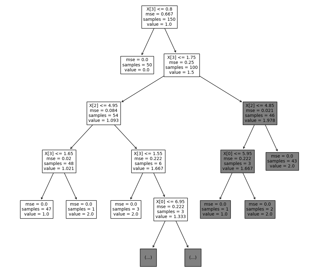
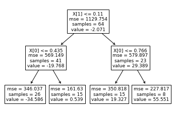
决策树可视化
Python
from sklearn.ensemble import RandomForestRegressor
from sklearn.datasets import make_regression

X, y = make_regression(n_features=4, n_informative=2, random_state=0, shuffle=False)
regr = RandomForestRegressor(max_depth=2, random_state=0)
regr.fit(X, y)

print(regr.predict([[0, 0, 0, 0]]))
# [-8.32987858]
调整决策树图片和字体大小
Python
from sklearn import tree
from sklearn.datasets import load_iris
import matplotlib.pyplot as plt

# load data
X, y = load_iris(return_X_y=True)

# create and train model
clf = tree.DecisionTreeClassifier(max_depth=4)  # set hyperparameter
clf.fit(X, y)

# plot tree
plt.figure(figsize=(12, 12))  # set plot size (denoted in inches)
tree.plot_tree(clf, fontsize=10)
plt.show()
plt.savefig("tree_high_dpi", dpi=100)