使用 sklearn 实现支持向量机分类算法
对银行客户流失数据进行特征筛选,构建 SVM 分类器,并与逻辑回归、决策树模型的分类效果进行对比。

Python
# 导入包
import pandas as pd
import numpy as np
import itertools
import seaborn as sns
import matplotlib.pyplot as plt
from matplotlib.ticker import FuncFormatter

plt.rcParams["font.sans-serif"] = ["SimHei"]
plt.rcParams["axes.unicode_minus"] = False
from scipy.stats import pearsonr
from sklearn.preprocessing import LabelEncoder
from sklearn.preprocessing import MinMaxScaler
from sklearn.feature_selection import VarianceThreshold
from sklearn.svm import SVC
from sklearn.linear_model import LogisticRegression
from sklearn.tree import DecisionTreeClassifier
from sklearn.metrics import classification_report
from sklearn import metrics
Python
# 读取数据
train = pd.read_excel("BankChurners2.xlsx", sheet_name="training")
test = pd.read_excel("BankChurners2.xlsx", sheet_name="testing")
x_train = train.drop(["Attrition_Flag"], axis=1)
y_train = train["Attrition_Flag"]
x_test = test.drop(["Attrition_Flag"], axis=1)
y_test = test["Attrition_Flag"]
变量编码
Python
# 提取文本类型的特征
text_features = [
    column for column in x_train.columns if x_train[column].dtype == "object"
]
# 对文本类型的特征进行编码
le = LabelEncoder()
for column in text_features:
    x_train[column] = le.fit_transform(train[column])
    x_test[column] = le.transform(test[column])
# 对标签进行编码
y_train.replace({"Existing Customer": 0, "Attrited Customer": 1}, inplace=True)
y_test.replace({"Existing Customer": 0, "Attrited Customer": 1}, inplace=True)
特征选择
移除低方差特征
Python
# 删除 id 列
x_train.drop(["id"], axis=1, inplace=True)
x_test.drop(["id"], axis=1, inplace=True)
# 将特征进行最小最大归一化
scaler = MinMaxScaler()
x_train = pd.DataFrame(
    scaler.fit_transform(x_train), index=x_train.index, columns=x_train.columns
)
x_test = pd.DataFrame(
    scaler.transform(x_test), index=x_test.index, columns=x_test.columns
)
# 移除低方差(归一化后方差小于 0.02)特征
selector = VarianceThreshold(threshold=0.02)
selector.fit(x_train)
# 打印因为低方差被移除的特征
print("因为低方差被移除特征:", x_train.columns[~selector.get_support()])
x_train = x_train.loc[:, selector.get_support()]
x_test = x_test.loc[:, selector.get_support()]
Text Only
因为低方差被移除特征: Index(['Total_Amt_Chng_Q4_Q1', 'Total_Ct_Chng_Q4_Q1'], dtype='object')
移除高相关特征中方差较低的那一个
Python
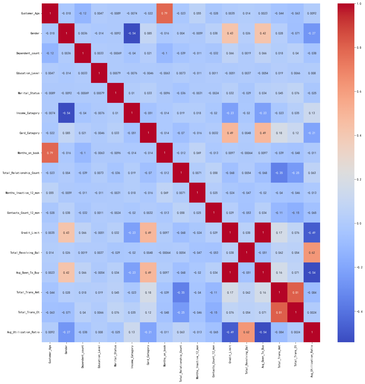
# 绘制特征之间的相关性热力图
plt.figure(figsize=(20, 20))
corr = x_train.corr()
sns.heatmap(corr, annot=True, cmap="coolwarm")
plt.show()
Python
# 打印相关性绝对值大于 0.8 的特征
corr = corr.abs()
corr = corr.where(np.triu(np.ones(corr.shape), k=1).astype(bool))
corr = corr.stack()
corr = corr[corr > 0.8]
print("相关性绝对值大于 0.8 的特征:", [i for i in corr.index])
# 从数据集中移除相关性绝对值大于 0.8 的特征中方差较小的特征
feature_to_remove = []
corr = corr.reset_index()
corr.columns = ["feature1", "feature2", "corr"]
for row in corr.itertuples():
    if x_train[row.feature1].var() < x_train[row.feature2].var():
        feature_to_remove.append(row.feature1)
    else:
        feature_to_remove.append(row.feature2)
feature_to_remove = list(set(feature_to_remove))
print("相关性绝对值大于 0.8 的特征中方差较小的特征:", feature_to_remove)
x_train.drop(feature_to_remove, axis=1, inplace=True)
x_test.drop(feature_to_remove, axis=1, inplace=True)
Text Only
相关性绝对值大于0.8的特征: [('Credit_Limit', 'Avg_Open_To_Buy'), ('Total_Trans_Amt', 'Total_Trans_Ct')]
相关性绝对值大于0.8的特征中方差较小的特征: ['Avg_Open_To_Buy', 'Total_Trans_Ct']
移除与标签相关性较低的特征
Python
# 移除与标签相关性绝对值小于 0.02 的特征
feature_to_remove = []
for i in x_train.columns:
    pearson_corr = pearsonr(x_train[i], y_train)[0]
    if abs(pearson_corr) < 0.02:
        feature_to_remove.append(i)
print("与标签相关性绝对值小于 0.02 的特征:", feature_to_remove)
x_train.drop(feature_to_remove, axis=1, inplace=True)
x_test.drop(feature_to_remove, axis=1, inplace=True)
Text Only
与标签相关性绝对值小于0.02的特征: ['Education_Level', 'Marital_Status', 'Income_Category', 'Card_Category', 'Months_on_book']
Text Only
最终选择的特征 ['Customer_Age' 'Gender' 'Dependent_count' 'Total_Relationship_Count'
 'Months_Inactive_12_mon' 'Contacts_Count_12_mon' 'Credit_Limit'
 'Total_Revolving_Bal' 'Total_Trans_Amt' 'Avg_Utilization_Ratio']
构建 SVM 分类器
Python
svm = SVC(kernel="poly")
svm.fit(x_train, y_train)
print("训练集准确率:%.2f%%" % (svm.score(x_train, y_train) * 100))
print("超平面的截距项 b 为{}".format(svm.intercept_[0]))
print("决策函数为{}".format(svm.decision_function(x_train)))
Text Only
训练集准确率: 88.04%
超平面的截距项b为-0.9575823695081735
决策函数为[-1.59427586 -1.8345902  -1.00014489 ... -1.60371229 -1.94589042
 -1.6133594 ]
在测试集上给出模型分类的效果
Python
def evaluate(true, pred):
    acc = metrics.accuracy_score(true, pred)
    presision = metrics.precision_score(true, pred)
    recall = metrics.recall_score(true, pred)
    f1 = metrics.f1_score(true, pred)
    print("整体分类误差率:{:.2%}".format(acc))
    print("Precision:{:.2%}".format(presision))
    print("Recall:{:.2%}".format(recall))
    print("F1 得分:{:.2%}".format(f1))
    return acc, presision, recall, f1
Python
# 在测试集上给出模型分类的效果
y_pred_svm = svm.predict(x_test)
print(classification_report(y_test, y_pred_svm))
acc_svm, presision_svm, recall_svm, f1_svm = evaluate(y_test, y_pred_svm)
Text Only
              precision    recall  f1-score   support

           0       0.89      0.99      0.93      2637
           1       0.82      0.32      0.46       490

    accuracy                           0.88      3127
   macro avg       0.85      0.66      0.70      3127
weighted avg       0.88      0.88      0.86      3127

整体分类误差率:88.26%
Precision:81.54%
Recall:32.45%
F1得分:46.42%
将 SVM 的结果与逻辑回归以及决策树结果进行对比分析
逻辑回归
Python
lr = LogisticRegression()
lr.fit(x_train, y_train)
# 测试集上的预测结果
y_pred_lr = lr.predict(x_test)
print(classification_report(y_test, y_pred_lr))
acc_lr, presision_lr, recall_lr, f1_lr = evaluate(y_test, y_pred_lr)
Text Only
              precision    recall  f1-score   support

           0       0.88      0.98      0.93      2637
           1       0.78      0.31      0.44       490

    accuracy                           0.88      3127
   macro avg       0.83      0.65      0.69      3127
weighted avg       0.87      0.88      0.85      3127

整体分类误差率:87.78%
Precision:77.55%
Recall:31.02%
F1得分:44.31%
决策树
Python
dt = DecisionTreeClassifier()
dt.fit(x_train, y_train)
# 测试集上的预测结果
y_pred_dt = dt.predict(x_test)
print(classification_report(y_test, y_pred_dt))
acc_dt, presision_dt, recall_dt, f1_dt = evaluate(y_test, y_pred_dt)
Text Only
              precision    recall  f1-score   support

           0       0.95      0.95      0.95      2637
           1       0.73      0.72      0.72       490

    accuracy                           0.91      3127
   macro avg       0.84      0.83      0.84      3127
weighted avg       0.91      0.91      0.91      3127

整体分类误差率:91.43%
Precision:73.12%
Recall:71.63%
F1得分:72.37%
绘制各模型在测试集上的训练效果
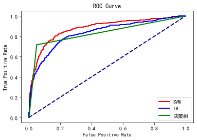
ROC 曲线
Python
# 绘制 ROC 曲线
# SVM 的 ROC 曲线
y_pred_proba_svm = svm.decision_function(x_test)
fpr_svm, tprr_svm, thresholdsr_svm = metrics.roc_curve(y_test, y_pred_proba_svm)
plt.plot(fpr_svm, tprr_svm, color="r", lw=2, label="SVM")
# 逻辑回归的 ROC 曲线
y_pred_proba_lr = lr.predict_proba(x_test)[:, 1]
fpr_lr, tprr_lr, thresholdsr_lr = metrics.roc_curve(y_test, y_pred_proba_lr)
plt.plot(fpr_lr, tprr_lr, color="b", lw=2, label="LR")
# 决策树的 ROC 曲线
y_pred_proba_dt = dt.predict_proba(x_test)[:, 1]
fpr_df, tpr_dt, thresholds_dt = metrics.roc_curve(y_test, y_pred_proba_dt)
plt.plot(fpr_df, tpr_dt, color="g", lw=2, label="决策树")

plt.plot([0, 1], [0, 1], color="navy", lw=2, linestyle="--")
plt.xlabel("False Positive Rate")
plt.ylabel("True Positive Rate")
plt.title("ROC Curve")
plt.legend(loc="lower right")
plt.show()
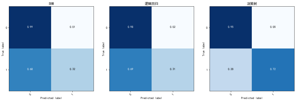
混淆矩阵
Python
# 绘制测试集上的混淆矩阵
def plot_confusion_matrix(
    cm, classes, normalize=False, title="Confusion matrix", cmap="Blues", colorbar=True
):
    """
    This function prints and plots the confusion matrix.
    Normalization can be applied by setting `normalize=True`.
    """
    if normalize:
        cm = cm.astype("float") / cm.sum(axis=1)[:, np.newaxis]

    plt.imshow(cm, interpolation="nearest", cmap=cmap)
    plt.title(title)
    if colorbar:
        plt.colorbar()
    tick_marks = np.arange(len(classes))
    plt.xticks(tick_marks, classes, rotation=45)
    plt.yticks(tick_marks, classes)

    fmt = ".2f" if normalize else "d"
    thresh = cm.max() / 2.0
    for i, j in itertools.product(range(cm.shape[0]), range(cm.shape[1])):
        plt.text(
            j,
            i,
            format(cm[i, j], fmt),
            horizontalalignment="center",
            color="white" if cm[i, j] > thresh else "black",
        )

    plt.tight_layout()
    plt.ylabel("True label")
    plt.xlabel("Predicted label")
Python
fig = plt.figure(figsize=(15, 5))
# SVM 的混淆矩阵
ax1 = fig.add_subplot(131)
cm_svm = metrics.confusion_matrix(y_test, y_pred_svm)
plot_confusion_matrix(
    cm_svm, classes=["0", "1"], normalize=True, title="SVM", colorbar=False
)
# 逻辑回归的混淆矩阵
ax2 = fig.add_subplot(132)
cm_lr = metrics.confusion_matrix(y_test, y_pred_lr)
plot_confusion_matrix(
    cm_lr, classes=["0", "1"], normalize=True, title="逻辑回归", colorbar=False
)
# 决策树的混淆矩阵
ax3 = fig.add_subplot(133)
cm_dt = metrics.confusion_matrix(y_test, y_pred_dt)
plot_confusion_matrix(
    cm_dt, classes=["0", "1"], normalize=True, title="决策树", colorbar=False
)
准确率、精确率、召回率、F1 值
Python
# 绘制模型的评价指标
def to_percent(temp, position):
    return "%1.0f" % (100 * temp) + "%"


fig = plt.figure(figsize=(15, 5))
ax1 = fig.add_subplot(131)
plt.bar(["SVM", "LR", "DT"], [acc_svm, acc_lr, acc_dt], color=["r", "b", "g"])
plt.gca().yaxis.set_major_formatter(FuncFormatter(to_percent))
plt.title("Accuracy")
plt.ylim(0.8, 1)
ax2 = fig.add_subplot(132)
plt.bar(
    ["SVM", "LR", "DT"],
    [presision_svm, presision_lr, presision_dt],
    color=["r", "b", "g"],
)
plt.gca().yaxis.set_major_formatter(FuncFormatter(to_percent))
plt.title("Presision")
plt.ylim(0.6, 1)
ax3 = fig.add_subplot(133)
plt.bar(["SVM", "LR", "DT"], [recall_svm, recall_lr, recall_dt], color=["r", "b", "g"])
plt.gca().yaxis.set_major_formatter(FuncFormatter(to_percent))
plt.title("Recall")
plt.show()