方差缩减技术之条件期望法
使用条件期望法降低蒙特卡洛模拟得到的估计量的方差。
Python
import pandas as pd
import numpy as np
import matplotlib.pyplot as plt
from tqdm import tqdm
from scipy.stats import gamma

np.random.seed(0)
问题描述

方差缩减技术——条件期望法
后验分布

Python
Number = np.array(
    [
        38,
        1,
        13,
        36,
        24,
        3,
        15,
        34,
        22,
        5,
        17,
        32,
        20,
        7,
        11,
        30,
        26,
        9,
        28,
        37,
        2,
        14,
        35,
        23,
        4,
        16,
        33,
        21,
        6,
        18,
        31,
        19,
        8,
        12,
        29,
        25,
        10,
        27,
    ]
)
Wheel1 = np.array(
    [
        2127,
        2082,
        2110,
        2221,
        2192,
        2008,
        2035,
        2113,
        2099,
        2199,
        2044,
        2133,
        1912,
        1999,
        1974,
        2051,
        1984,
        2053,
        2019,
        2046,
        1999,
        2168,
        2150,
        2041,
        2047,
        2091,
        2142,
        2196,
        2153,
        2191,
        2192,
        2284,
        2136,
        2110,
        2032,
        2188,
        2121,
        2158,
    ]
)
wheel2 = np.array(
    [
        1288,
        1234,
        1261,
        1251,
        1164,
        1438,
        1264,
        1335,
        1342,
        1232,
        1326,
        1302,
        1227,
        1192,
        1278,
        1336,
        1296,
        1298,
        1205,
        1189,
        1171,
        1279,
        1315,
        1296,
        1256,
        1304,
        1304,
        1351,
        1281,
        1392,
        1306,
        1330,
        1266,
        1224,
        1190,
        1229,
        1320,
        1336,
    ]
)
wheel = pd.DataFrame({"Wheel1": Wheel1, "Wheel2": wheel2}, index=Number)
wheel.sort_index(inplace=True)
Wheel 1
自然的 Monte Carlo 方法
模拟 Dirichlet 分布的随机数
计算\(\mu\)的估计值及其\(95\%\)置信区间
Python
def naive_nonte_carlo(n):
    df = pd.DataFrame(np.random.dirichlet(wheel["Wheel1"], size=n), columns=wheel.index)
    df["p19>max(pi)"] = df.apply(lambda x: x[19] > max(x[x.index != 19]), axis=1)
    mu = df["p19>max(pi)"].mean()
    return mu
Python
mu_list_maive_monte_carlo = []
for simulation in tqdm(range(1000)):
    mu = naive_nonte_carlo(n)
    mu_list_maive_monte_carlo.append(mu)
Text Only
100%|██████████| 1000/1000 [00:12<00:00, 78.60it/s]
Python
mu_mean_maive_monte_carlo = np.mean(mu_list_maive_monte_carlo)
mu_std_maive_monte_carlo = np.std(mu_list_maive_monte_carlo)
left = mu_mean_maive_monte_carlo - 1.96 * mu_std_maive_monte_carlo
right = mu_mean_maive_monte_carlo + 1.96 * mu_std_maive_monte_carlo
print("mu 的估计值为:{:.4f}".format(mu_mean_maive_monte_carlo))
print("95% 置信水平的置信区间为:({:.4f}, {:.4f})".format(left, right))
Text Only
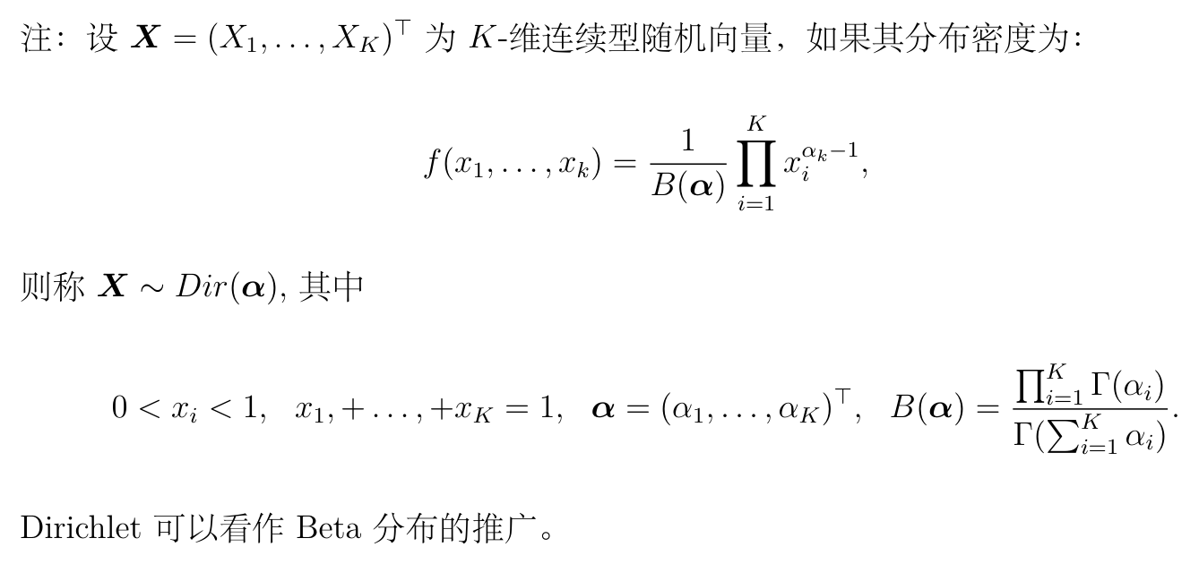
mu的估计值为:0.6318
95%置信水平的置信区间为:(0.5378, 0.7259)
画出 Monte Carlo 估计的直方图
Python
fig = plt.figure(figsize=(8, 8))
ax = fig.add_subplot(111)
plt.hist(mu_list_maive_monte_carlo)
ax.set_xlabel(r"$\mu$")
ax.set_ylabel("Frequency")
plt.show()
条件期望法
这里有点疑问,我不知道怎么计算当给定\(p^{19}\)时,其他\(p\)小于\(p^{19}\)的条件期望。代码中用的是独立分布的 CDF 值相乘,但实际上各个变量之间是相关的,并不是独立分布的。
对每一个 wheel_19,求条件期望
Python
def less_than_q19():
    # 用 gamma 分布生成 wheel_19
    wheel_19 = np.random.gamma(shape=wheel["Wheel1"][19] + 1)
    less_than_q19 = 1
    # 对每一个 q_i,生成 gamma 分布,然后计算 wheel_i<wheel_19 的概率
    for i in range(1, 38 + 1):
        if i != 19:
            wheel_i_less_than_q19 = gamma.cdf(wheel_19, wheel["Wheel1"][i] + 1)
            less_than_q19 *= wheel_i_less_than_q19
    return less_than_q19
Python
mu_list_conditional_expectation = []
for simulation in tqdm(range(1000)):
    less_than_q19_list = []
    for i in range(n):
        less_than_q19_value = less_than_q19()
        less_than_q19_list.append(less_than_q19_value)
    mu = np.mean(less_than_q19_list)
    mu_list_conditional_expectation.append(mu)
Text Only
100%|██████████| 1000/1000 [09:27<00:00, 1.76it/s]
计算\(\mu\)的估计值及其\(95\%\)置信区间
Python
mu_mean_conditional_expectation = np.mean(mu_list_conditional_expectation)
mu_std_conditional_expectation = np.std(mu_list_conditional_expectation)
left = mu_mean_conditional_expectation - 1.96 * mu_std_conditional_expectation
right = mu_mean_conditional_expectation + 1.96 * mu_std_conditional_expectation
print("mu 的估计值为:{:.4f}".format(mu_mean_conditional_expectation))
print("95% 置信水平的置信区间为:({:.4f}, {:.4f})".format(left, right))
Text Only
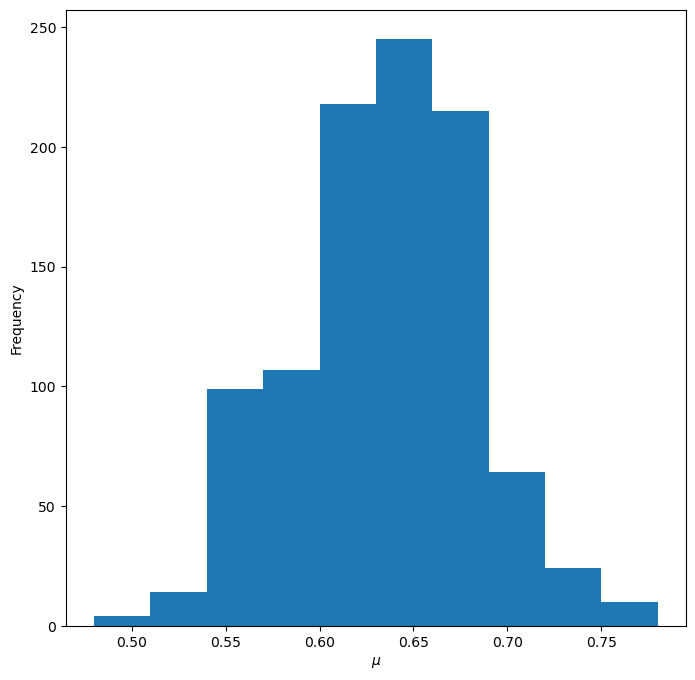
mu的估计值为:0.6299
95%置信水平的置信区间为:(0.5631, 0.6968)
画出条件期望法估计的直方图
Python
fig = plt.figure(figsize=(8, 8))
ax = fig.add_subplot(111)
plt.hist(mu_list_conditional_expectation)
ax.set_xlabel(r"$\mu$")
ax.set_ylabel("Frequency")
plt.show()

比较两种方法的方差
Python
print("自然的 Monte Carlo 方法的估计值的方差为:{:.4f}".format(mu_std_maive_monte_carlo))
print("条件期望法的估计值的方差为:{:.4f}".format(mu_std_conditional_expectation))
Text Only
自然的Monte Carlo方法的估计值的方差为:0.0480
条件期望法的估计值的方差为:0.0341
条件期望法的结果比自然的 Monte Carlo 方法的方差更小。
Wheel 2
自然的 Monte Carlo 方法
模拟 Dirichlet 分布的随机数
计算\(\mu\)的估计值及其\(95\%\)置信区间
Python
def naive_nonte_carlo(n):
    df = pd.DataFrame(np.random.dirichlet(wheel["Wheel2"], size=n), columns=wheel.index)
    df["p3>max(pi)"] = df.apply(lambda x: x[3] > max(x[x.index != 3]), axis=1)
    mu = df["p3>max(pi)"].mean()
    return mu
Python
mu_list_maive_monte_carlo = []
for simulation in tqdm(range(1000)):
    mu = naive_nonte_carlo(n)
    mu_list_maive_monte_carlo.append(mu)
Text Only
100%|██████████| 1000/1000 [00:14<00:00, 70.42it/s]
Python
mu_mean_maive_monte_carlo = np.mean(mu_list_maive_monte_carlo)
mu_std_maive_monte_carlo = np.std(mu_list_maive_monte_carlo)
left = mu_mean_maive_monte_carlo - 1.96 * mu_std_maive_monte_carlo
right = mu_mean_maive_monte_carlo + 1.96 * mu_std_maive_monte_carlo
print("mu 的估计值为:{:.4f}".format(mu_mean_maive_monte_carlo))
print("95% 置信水平的置信区间为:({:.4f}, {:.4f})".format(left, right))
Text Only
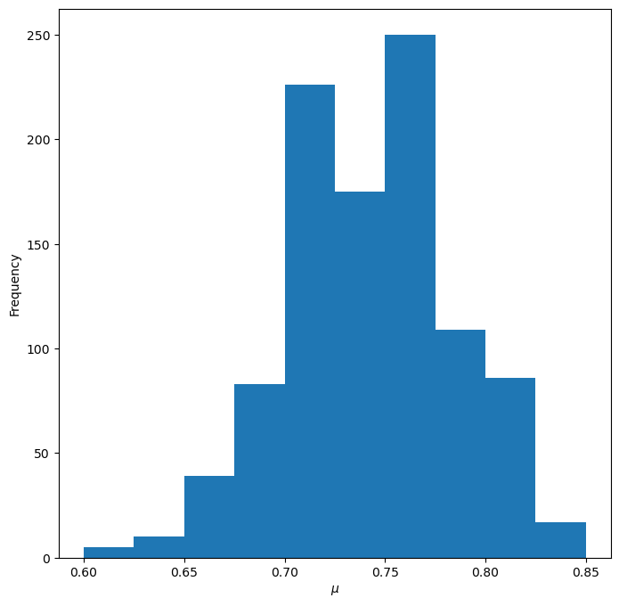
mu的估计值为:0.7401
95%置信水平的置信区间为:(0.6578, 0.8224)
画出 Monte Carlo 估计的直方图
Python
fig = plt.figure(figsize=(8, 8))
ax = fig.add_subplot(111)
plt.hist(mu_list_maive_monte_carlo)
ax.set_xlabel(r"$\mu$")
ax.set_ylabel("Frequency")
plt.show()
条件期望法
对每一个 wheel_3,求条件期望
Python
def less_than_q3():
    # 用 gamma 分布生成 wheel_3
    wheel_3 = np.random.gamma(shape=wheel["Wheel2"][3] + 1)
    less_than_q3 = 1
    # 对每一个 q_i,生成 gamma 分布,然后计算 wheel_i<wheel_3 的概率
    for i in range(1, 38 + 1):
        if i != 3:
            wheel_i_less_than_q3 = gamma.cdf(wheel_3, wheel["Wheel2"][i] + 1)
            less_than_q3 *= wheel_i_less_than_q3
    return less_than_q3
Python
mu_list_conditional_expectation = []
for simulation in tqdm(range(1000)):
    less_than_q3_list = []
    for i in range(n):
        less_than_q3_value = less_than_q3()
        less_than_q3_list.append(less_than_q3_value)
    mu = np.mean(less_than_q3_list)
    mu_list_conditional_expectation.append(mu)
Text Only
100%|██████████| 1000/1000 [08:54<00:00, 1.87it/s]
计算\(\mu\)的估计值及其\(95\%\)置信区间
Python
mu_mean_conditional_expectation = np.mean(mu_list_conditional_expectation)
mu_std_conditional_expectation = np.std(mu_list_conditional_expectation)
left = mu_mean_conditional_expectation - 1.96 * mu_std_conditional_expectation
right = mu_mean_conditional_expectation + 1.96 * mu_std_conditional_expectation
print("mu 的估计值为:{:.4f}".format(mu_mean_conditional_expectation))
print("95% 置信水平的置信区间为:({:.4f}, {:.4f})".format(left, right))
Text Only
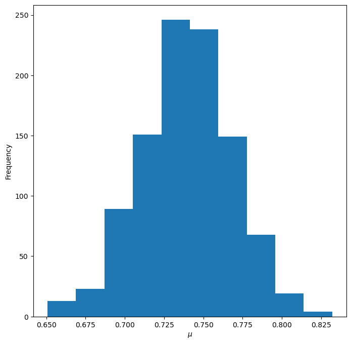
mu的估计值为:0.7393
95%置信水平的置信区间为:(0.6828, 0.7959)
画出条件期望法估计的直方图
Python
fig = plt.figure(figsize=(8, 8))
ax = fig.add_subplot(111)
plt.hist(mu_list_conditional_expectation)
ax.set_xlabel(r"$\mu$")
ax.set_ylabel("Frequency")
plt.show()
比较两种方法的方差
Python
print("自然的 Monte Carlo 方法的估计值的方差为:{:.4f}".format(mu_std_maive_monte_carlo))
print("条件期望法的估计值的方差为:{:.4f}".format(mu_std_conditional_expectation))
Text Only
自然的Monte Carlo方法的估计值的方差为:0.0420
条件期望法的估计值的方差为:0.0288
条件期望法的结果比自然的 Monte Carlo 方法的方差更小。