蒙特卡洛模拟的应用
使用蒙特卡洛方法实现模拟销售利润、计算二重积分以及重要性抽样。
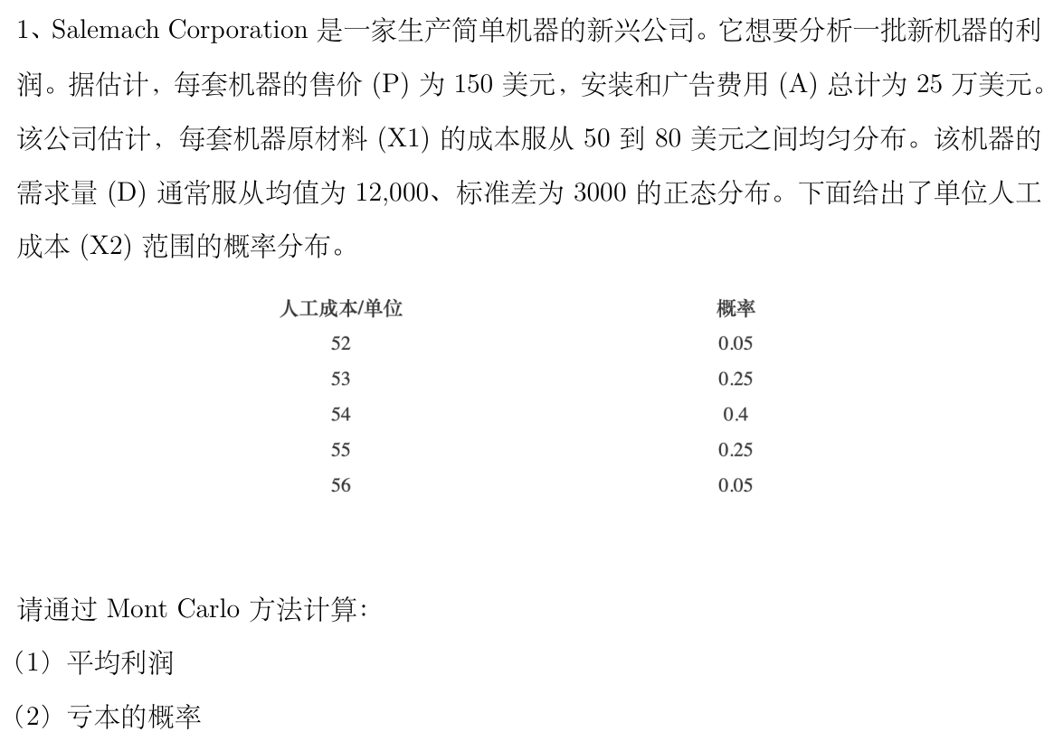
蒙特卡洛模拟销售利润
定义随机模拟次数和随机种子
构造随机数
# 定义函数,生成 X_2
def gen_X2():
    u = np.random.uniform(0, 1)
    if u <= 0.4:
        return 54
    elif u <= 0.65:
        return 53
    elif u <= 0.9:
        return 55
    elif u <= 0.95:
        return 52
    else:
        return 56
# 新建数据框,存放各变量
df = pd.DataFrame(
    columns=["P", "X1", "X2", "D", "A", "Profit"], index=range(num_simulation)
)
df["P"] = 150
df["A"] = 250000
df["X1"] = np.random.uniform(50, 80, num_simulation)
df["X2"] = [gen_X2() for i in range(num_simulation)]
df["D"] = np.random.normal(12000, 3000, num_simulation)
| P | X1 | X2 | D | A | Profit | |
|---|---|---|---|---|---|---|
| 0 | 150 | 66.464405 | 53 | 13285.544352 | 250000 | 155682.000137 |
| 1 | 150 | 71.455681 | 52 | 7841.598823 | 250000 | -41850.099314 |
| 2 | 150 | 68.082901 | 53 | 8691.266287 | 250000 | 1326.205206 |
| 3 | 150 | 66.346495 | 54 | 7103.369929 | 250000 | -39360.187767 |
| 4 | 150 | 62.709644 | 53 | 6853.320764 | 250000 | -14997.191074 |
| ... | ... | ... | ... | ... | ... | ... |
| 99995 | 150 | 71.777633 | 54 | 13766.849405 | 250000 | 83465.683781 |
| 99996 | 150 | 65.225615 | 54 | 13945.705918 | 250000 | 179170.520949 |
| 99997 | 150 | 74.303985 | 54 | 19177.595239 | 250000 | 166077.391728 |
| 99998 | 150 | 66.530968 | 54 | 12577.591120 | 250000 | 120649.431015 |
| 99999 | 150 | 56.772676 | 55 | 13833.015923 | 250000 | 278799.185933 |
100000 rows × 6 columns
计算平均利润和亏损的概率
average_profit = df["Profit"].mean()
print("平均利润为:{:.2f}美元".format(average_profit))
probability_of_loss = (df["Profit"] < 0).sum() / num_simulation
print("亏损概率为:{:.2%}".format(probability_of_loss))
平均利润为:121736.51美元
亏损概率为:21.55%
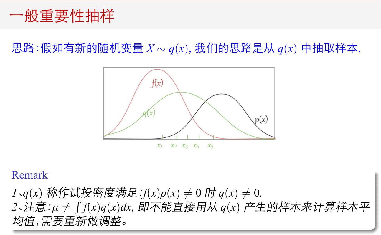
重要性抽样
要解决的问题
对于\(X \sim p(x)\),要求
问题 1:\(p(x)\)很难抽取,因此很难通过普通的随机模拟方法求解。
问题 2:\(f(x)\)和\(p(x)\)差异很大,体现在:当\(p(x)\)很大时,\(f(x)\)很小,而当当\(p(x)\)很小时,\(f(x)\)很大。这时,普通的随机模拟方法求解的结果很不准确。
基本思想
找到一个函数\(q(x)\),且当\(f(x)p(x)\ne 0\)时,\(q(x)\ne 0\),即当积分不为 0 时,\(q(x)\)也不能为 0。
这时,可以用下面的公式计算\(\mu\):
只需要对\(q(x)\)进行随机抽样,就可以计算出\(\mu\)。
如果\(q(x)\)抽样很容易,那么就可以让求\(\mu\)的过程更加简单。
用\(q(x)\)来计算\(\mu\)的公式为:
并且,可以证明,
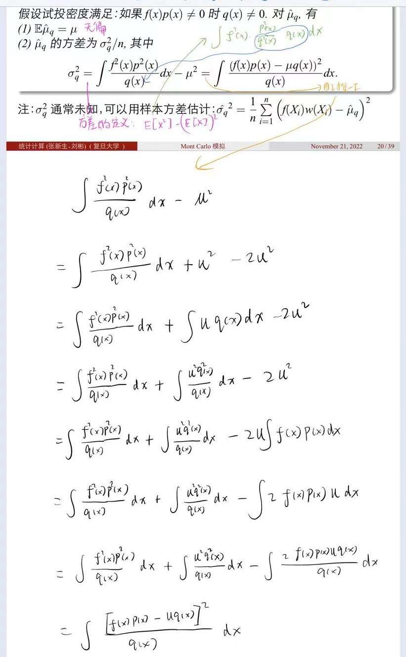
因此,当 $$ \bar{q}(x) \propto|f(x)| p(x) / c $$ \(\hat{\mu}_q\)的估计误差会较小。
选取试投密度时的三个要求
- 要求当 \(f(x)p(x) \ne 0\) 时,\(q(x) \ne 0\)
否则,在\(f(x)\)不为 0,且\(p(x)\)为正时,被积函数不为 0,但是\(q(x)\)为 0,说明永远也抽不到这个点。因此,\(\mu\)的估计值会偏小。
- \(q(x)\) 形状尽量与 \(|f(x)| p(x)\) 接近
因为
当 \(q(x)\) 形状与 \(|f(x)| p(x)\) 接近时,\(\sigma_q^2\)会较小。
- 当 \(x\) 趋于无穷时,要求 \(p(x)=o(g(x))\)
仍然是由于
若 \(p(x)\) 比\(g(x)\)更高阶,则\(\sigma_q^2\)会趋于无穷大。
随机模拟法计算二重积分
用随机模拟法计算二重积分 $$ I=\int_0^1 \int_0^1 e{x2+y^2} d x d y $$
并给出相应的区间估计。
# 设定随机种子
np.random.seed(0)


def f(x, y):
    return np.exp((x**2) + (y**2))


f_list = []
for i in range(100000):
    x = np.random.uniform(0, 1)
    y = np.random.uniform(0, 1)
    f_list.append(f(x, y))
intergral = np.mean(f_list)
sigma_intergral = (1 - 0) * np.std(f_list) / (np.sqrt(100000))
left = intergral - 1.96 * sigma_intergral
right = intergral + 1.96 * sigma_intergral
print("积分值为:{:.4f}".format(intergral))
print("95% 置信水平的置信区间为:({:.4f}, {:.4f})".format(left, right))
积分值为:2.1438
95%置信水平的置信区间为:(2.1376, 2.1501)
重要性抽样计算积分
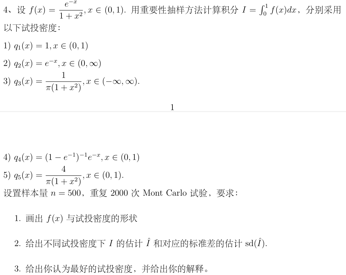
def f(x):
    return np.exp(-x) / (1 + x**2)


def q_1(x):
    return 1


def q_2(x):
    return np.exp(-x)


def q_3(x):
    return 1 / (np.pi * (1 + x**2))


def q_4(x):
    return (1 - np.exp(-1)) ** (-1) * np.exp(-x)


def q_5(x):
    return 4 / (np.pi * (1 + x**2))
画出 \(f(x)\) 与试投密度的形状
import matplotlib.pyplot as plt

plt.rcParams["font.size"] = 18
plt.rcParams["text.usetex"] = True
fig = plt.figure(figsize=(10, 8))
ax = fig.add_subplot(111)
x = np.linspace(0, 1, 1000)
for fun in [f, q_1, q_2, q_3, q_4, q_5]:
    y = [fun(i) for i in x]
    ax.plot(x, y, label=r"${}$".format(fun.__name__))
ax.set_xlabel(r"$x$")
ax.set_ylabel(r"Function Value", usetex=False)
ax.legend()
plt.show()

# 观察到所有函数在 0 到 1 上均小于 1.7,因此可以用舍选法生成样本
def gen_sample(fun, num_sample):
    sample = []
    while len(sample) < num_sample:
        x = np.random.uniform(0, 1)
        u = np.random.uniform(0, 1.7)
        if u <= fun(x):
            sample.append(x)
    return sample
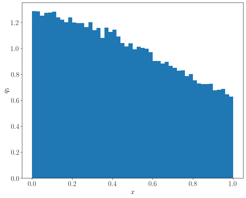
以\(q_5\)为例,检验生成的样本与原密度函数是否接近
fig = plt.figure(figsize=(10, 8))
ax = fig.add_subplot(111)
plt.hist(gen_sample(q_5, 100000), bins=50, density=True)
ax.set_xlabel(r"$x$")
ax.set_ylabel(r"$q_5$")
plt.show()
重要性抽样
n = 500
n_monte_carlo = 2000

for q in [q_1, q_2, q_3, q_4, q_5]:
    intergral_list = []
    for monte_carlo in range(n_monte_carlo):
        sample = gen_sample(q, n)
        # 如果 q 函数的定义域不是 (0, 1),则需要用自正则化抽样
        if q.__name__[-1] in ["2", "3"]:
            # 求 q 自身在 0 到 1 上的积分,下一步需要将 q(i) 除以这个积分,得到 q 在 0 到 1 上的概率密度函数
            q_density = np.mean([q(i) for i in sample])
        else:
            q_density = 1
        intergral = np.mean([f(i) / (q(i) / q_density) for i in sample])
        intergral_list.append(intergral)
    intergral_mean = np.mean(intergral_list)
    intergral_std = np.std(intergral_list)
    print("{}的积分值的估计为:{:.4f}".format(q.__name__, intergral_mean))
    print("{}的积分值的标准差的估计为:{:.4f}".format(q.__name__, intergral_std))
q_1的积分值的估计为:0.5251
q_1的积分值的标准差的估计为:0.0109
q_2的积分值的估计为:0.5676
q_2的积分值的标准差的估计为:0.0116
q_3的积分值的估计为:0.5468
q_3的积分值的标准差的估计为:0.0108
q_4的积分值的估计为:0.5250
q_4的积分值的标准差的估计为:0.0044
q_5的积分值的估计为:0.5250
q_5的积分值的标准差的估计为:0.0064
最优的试投函数
最好的试投函数是\(q_4\),因为它的估计误差最小。
这是由于\(q_4\)的形状与\(f(x)\)的形状接近,且\(q_4\)在\((0, 1)\)上的积分值为 1,不需要使用自正则化。
其他的试投密度中,\(q_2\)和\(q_3\)的定义域不是\((0, 1)\),因此需要使用自正则化。这会导致估计误差增大。
\(q_1\)虽然不需要使用自正则化,但是它的形状与\(f(x)\)的形状不接近,因此估计误差也较大。
\(q_5\)也是一个不错的试投函数,它不需要使用自正则化,且形状与\(f(x)\)的形状接近,但没有\(q_4\)更接近。