使用 sklearn 实现决策树分类算法
基于 Information Value 对类别特征进行初步筛选,使用 sklearn 实现决策树分类算法,对客户流失情况进行分类预测,汇报 Accuracy、Presicion、Recall、F1、AUC 等评价指标。
导入包和数据
Python
# 导入包
import pandas as pd
import numpy as np
import seaborn as sb
import matplotlib.pyplot as plt
from sklearn import preprocessing
from sklearn.tree import DecisionTreeClassifier
from sklearn.model_selection import cross_val_score
import sklearn.metrics as metrics
Python
# 导入数据
train = pd.read_excel("BankChurners2.xlsx", sheet_name="training", engine="openpyxl")
test = pd.read_excel("BankChurners2.xlsx", sheet_name="testing", engine="openpyxl")
x_train = train.drop(columns=["id", "Attrition_Flag"])
x_test = test.drop(columns=["id", "Attrition_Flag"])
y_train = train["Attrition_Flag"]
y_test = test["Attrition_Flag"]
查看数据
Text Only
##    Customer_Age Gender  ...  Total_Ct_Chng_Q4_Q1 Avg_Utilization_Ratio
## 0            46      M  ...                0.559                 0.289
## 1            58      M  ...                0.778                 0.088
## 2            47      M  ...                1.357                 0.000
## 3            54      M  ...                0.423                 0.000
## 4            44      F  ...                0.667                 0.000
##
## [5 rows x 19 columns]
Text Only
## 0    Existing Customer
## 1    Existing Customer
## 2    Existing Customer
## 3    Attrited Customer
## 4    Existing Customer
## Name: Attrition_Flag, dtype: object
特征筛选
绘制相关系数热力图,识别特征之间的相关性
Python
# 生成相关系数矩阵
corr = x_train.corr()
# 生成上三角形矩阵,在后面可以用 mask 把上三角形的相关系数覆盖住
matrix = np.triu(corr)
# 设置图片大小
fig, ax = plt.subplots(figsize=(20, 10))
# 生成热力图。cmap 是颜色,annot 是是否显示相关系数,mask 是上三角形矩阵
sb.heatmap(corr, cmap="Blues", annot=True, mask=matrix)
plt.show()
Python
fig, ax = plt.subplots(figsize=(5, 5))
plt.scatter(x_train["Credit_Limit"], x_train["Avg_Open_To_Buy"])
plt.show()
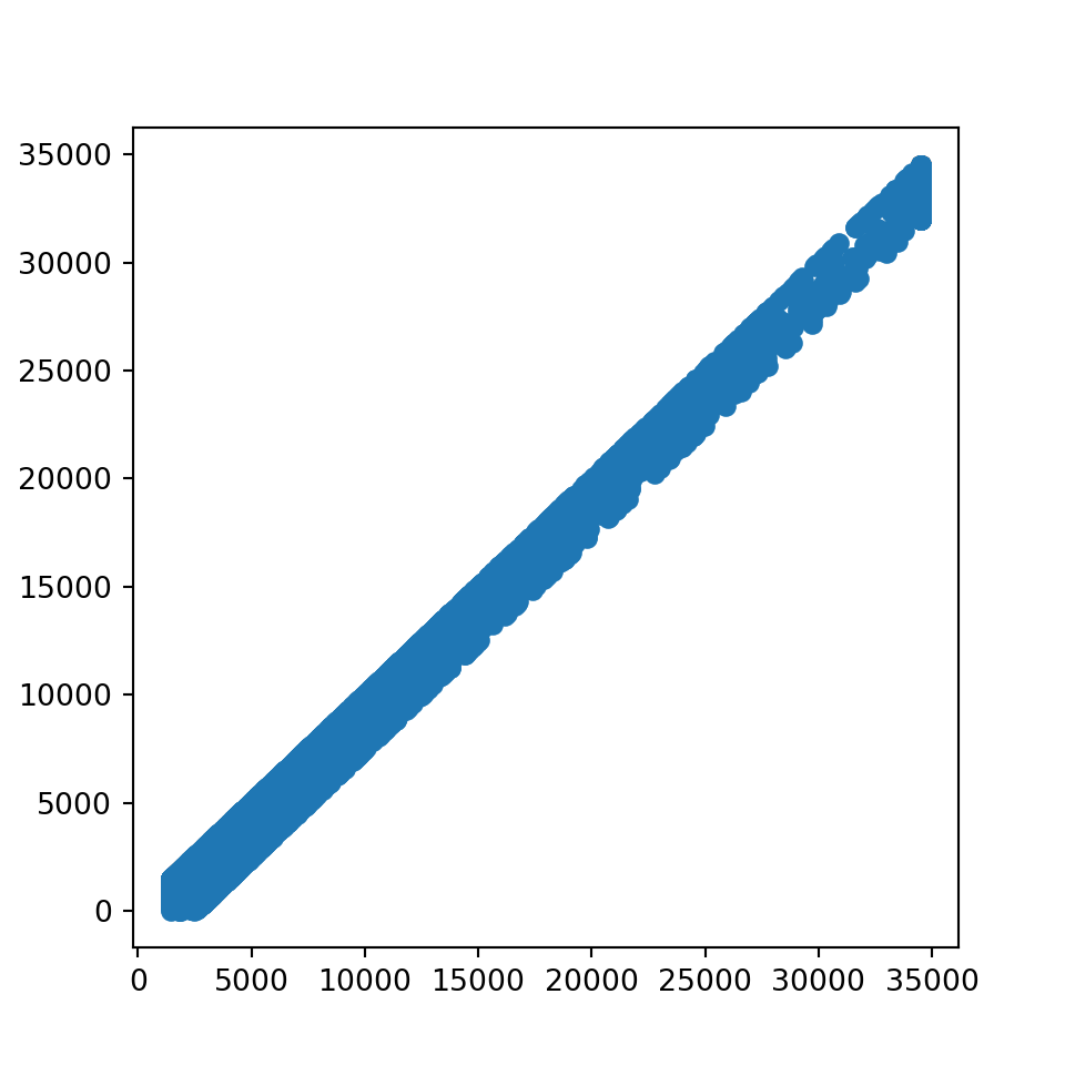
Python
# 由于 Avg_Open_To_Buy 和 Credit_Limit 相关非常高,故删除 Avg_Open_To_Buy
x_train = x_train.drop(columns=["Avg_Open_To_Buy"])
x_test = x_test.drop(columns=["Avg_Open_To_Buy"])
Python
# 离散变量
discrete_features = [
    "Gender",
    "Dependent_count",
    "Education_Level",
    "Marital_Status",
    "Income_Category",
    "Card_Category",
    "Total_Relationship_Count",
    "Months_Inactive_12_mon",
    "Contacts_Count_12_mon",
]
# 连续变量
continuous_features = x_train.columns.drop(discrete_features)
对离散分组变量,计算 Information Value,对特征进行筛选。
Python
def cal_IV(feature, label):
    # 计算 WOE
    woe = pd.crosstab(feature, label, normalize="columns").assign(
        woe=lambda dfx: np.log(dfx["Attrited Customer"] / dfx["Existing Customer"])
    )
    # 计算 IV
    iv = np.sum(woe["woe"] * (woe["Attrited Customer"] - woe["Existing Customer"]))
    return iv
Python
# 存放各变量的 IV 值
iv_dict = {}
for feature in discrete_features:
    iv_dict[feature] = cal_IV(x_train[feature], y_train)
Text Only
## {'Card_Category': 0.0013000619131457577, 'Marital_Status': 0.0036967489569619365, 'Gender': 0.003925134588828062, 'Income_Category': 0.009186000687735793, 'Education_Level': 0.010361108736073923, 'Dependent_count': 0.011508555906514393, 'Total_Relationship_Count': 0.17613730345552436, 'Months_Inactive_12_mon': 0.375963833865356, 'Contacts_Count_12_mon': inf}
Python
# 由于 Card_Category 的 IV 值非常低,故删除 Card_Category
discrete_features.remove("Card_Category")
x_train = x_train.drop(columns=["Card_Category"])
x_test = x_test.drop(columns=["Card_Category"])
将文本型的特征和标签编码成数值型
Python
# 将特征转换为数值型
OrdinalEncoder = preprocessing.OrdinalEncoder()
x_train = OrdinalEncoder.fit_transform(x_train[discrete_features])
x_test = OrdinalEncoder.transform(x_test[discrete_features])
Python
# 将标签转换为数值型
le = preprocessing.LabelEncoder()
y_train = le.fit_transform(y_train)
y_test = le.transform(y_test)
构建决策树
基于交叉验证选择最优的树深度
Python
# 基于交叉验证选择最优的树深度
depths = np.arange(1, 20)
scores = []
for depth in depths:
    clf = DecisionTreeClassifier(max_depth=depth, random_state=42)
    score = cross_val_score(clf, x_train, y_train, cv=5).mean()
    scores.append(score)
绘制树深度与准确率的关系
Python
# 绘制树深度与准确率的关系
plt.plot(depths, scores)
plt.annotate(
    "best depth: {}".format(depths[np.argmax(scores)]),
    xy=(depths[np.argmax(scores)], np.max(scores)),
    xytext=(np.argmax(scores) + 1, np.max(scores) - 0.02),
    arrowprops=dict(facecolor="black", shrink=0.05),
)
plt.xlabel("depth")
plt.ylabel("score")
plt.show()

选择最优的树深度,构建决策树
Python
# 选择最优的树深度,构建决策树
clf = DecisionTreeClassifier(max_depth=depths[np.argmax(scores)], random_state=42)
# 训练模型
clf.fit(x_train, y_train)
# 预测标签
Python
y_pred = clf.predict(x_test)
# 预测标签的概率
y_pred_proba = clf.predict_proba(x_test)[:, 1]
y_pred_proba
模型评价
Accuracy, Presicion, Recall, F1
Python
# 计算准确率 Accuracy
accuracy = np.sum(y_pred == y_test) / len(y_test)
# 计算精确率 Presicion
presicion = np.sum(y_pred[y_pred == 1] == y_test[y_pred == 1]) / np.sum(y_pred == 1)
# 计算召回率 Recall
recall = np.sum(y_pred[y_test == 1] == y_test[y_test == 1]) / np.sum(y_test == 1)
# 计算 F1 值
f1 = 2 * presicion * recall / (presicion + recall)
Python
print(
    "Accuracy: {:.2%}\n\
Presicion: {:.2%}\n\
Recall: {:.2%}\n\
F1: {:.2%}".format(
        accuracy, presicion, recall, f1
    )
)
使用 sklearn 自带的评价指标函数
Python
print(
    "Accuracy: {:.2%}\n\
Presicion: {:.2%}\n\
Recall: {:.2%}\n\
F1: {:.2%}".format(
        metrics.accuracy_score(y_test, y_pred),
        metrics.precision_score(y_test, y_pred),
        metrics.recall_score(y_test, y_pred),
        metrics.f1_score(y_test, y_pred),
    )
)
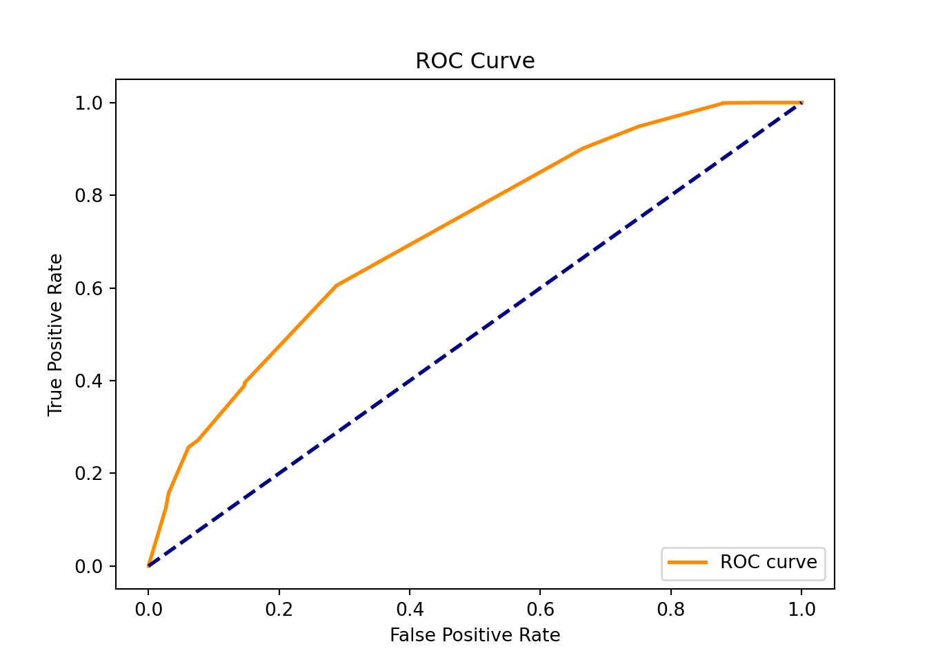
绘制 ROC 曲线
Python
# 绘制 ROC 曲线
fpr, tpr, thresholds = metrics.roc_curve(y_test, y_pred_proba)
plt.plot(fpr, tpr, color="darkorange", lw=2, label="ROC curve")
plt.plot([0, 1], [0, 1], color="navy", lw=2, linestyle="--")
plt.xlabel("False Positive Rate")
plt.ylabel("True Positive Rate")
plt.title("ROC Curve")
plt.legend(loc="lower right")
plt.show()