随机抽样之 MCMC 算法
MCMC 算法是一种随机抽样算法。借助建议分布,可以在各个样本状态之间进行转移,最终得到目标分布的样本。本文使用了逐分量 MCMC、随机游走和独立性抽样构造 Ising 分布和二元正态分布的随机样本。
Python
# 导入包
import numpy as np

# 设置随机数种子
np.random.seed(0)
from scipy.stats import multivariate_normal
import matplotlib.pyplot as plt

plt.rcParams["font.sans-serif"] = ["simsun"]
plt.rcParams["axes.unicode_minus"] = False
from tqdm import tqdm
Ising 模型
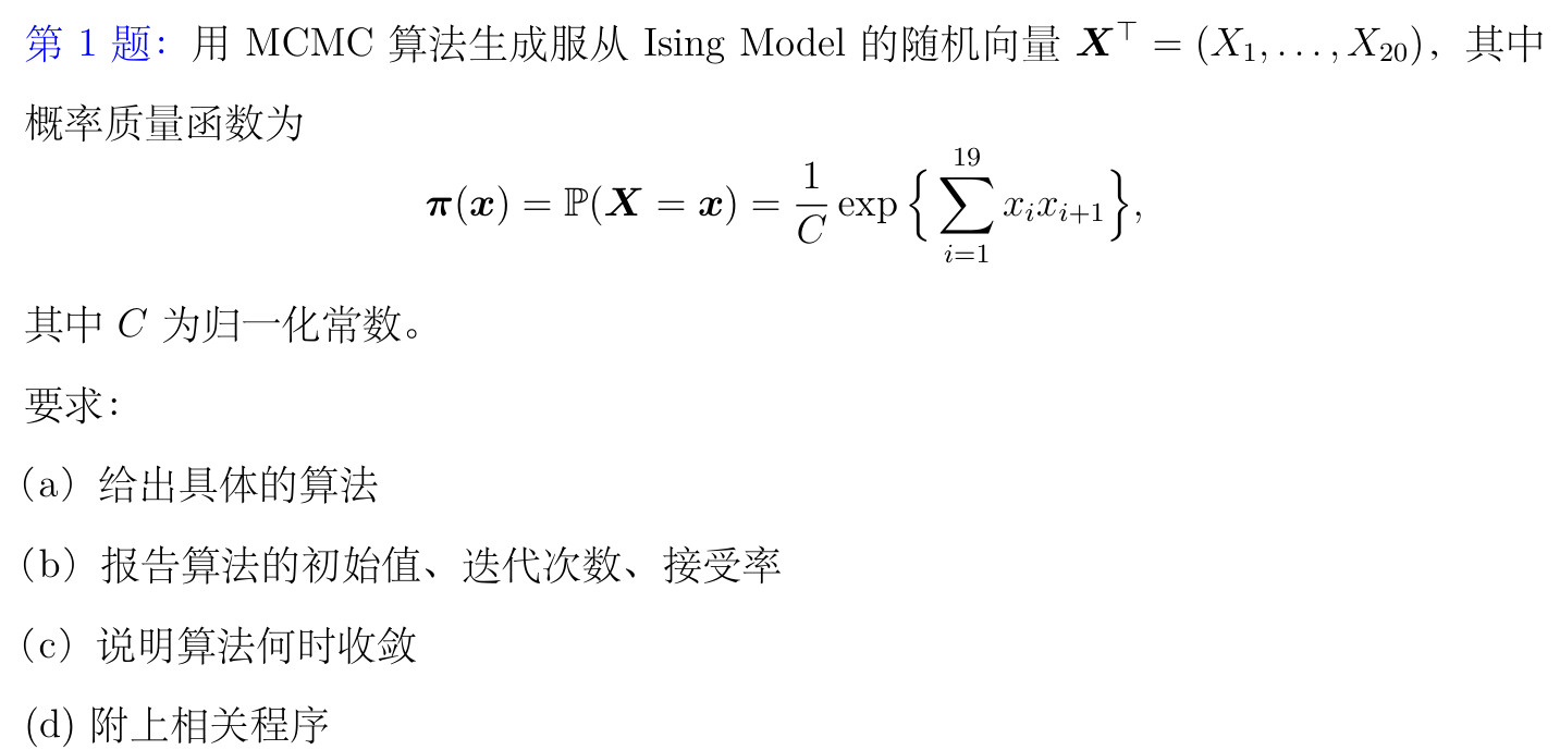
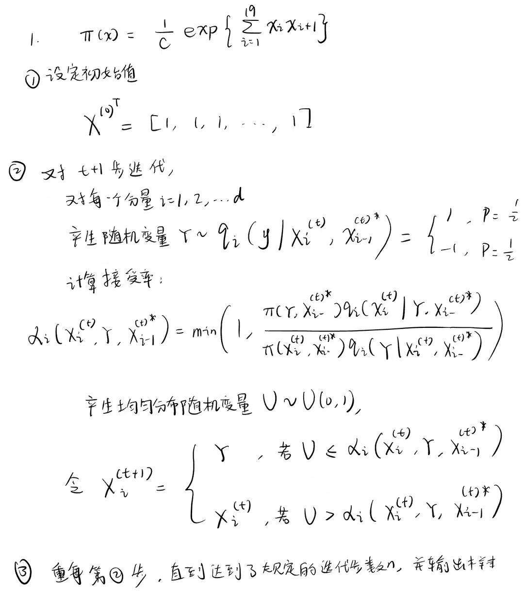
算法
定义目标分布的概率密度函数
Python
def pi(vector_x):
    sum_x_i__times_x_i_plus_1 = 0
    for i in range(len(vector_x) - 1):
        sum_x_i__times_x_i_plus_1 += vector_x[i] * vector_x[i + 1]
    return np.exp(sum_x_i__times_x_i_plus_1)
定义接受率函数
逐分量 Metropolis-Hastings 算法
初始化样本
Python
# 生成初始向量
vector_x = np.random.randint(2, size=20)
# 将 vector_x 中的 0 替换为 -1
vector_x[vector_x == 0] = -1
# 打印初始向量
print("初始向量为:", vector_x)
Text Only
初始向量为: [ 1 1 -1 -1 -1 -1 -1 -1 -1 -1 1 1 -1 -1 1 -1 -1 1 -1 1]
设定迭代次数
迭代产生样本
Python
# 不断迭代,生成数量为 iteration 的样本
for t in tqdm(range(iteration)):
    # 逐分量更新
    for i in range(d):
        # 生成一个随机数 y,它来自试投密度函数:y 有 0.5 的概率取值为 1,有 0.5 的概率取值为 -1
        u = np.random.uniform(0, 1)
        if u < 0.5:
            y = 1
        else:
            y = -1
        # 基于接受率,决定是否接受
        vector_y_x_i_ = vector_x.copy()
        # 将 x_i 的值改为 y
        vector_y_x_i_[i] = y
        # q(x_i | y, x_{i-}) 和 q(y | x_i, x_{i-}) 的值均为 0.5,可以自动约去
        alpha_i = alpha(vector_x, vector_y_x_i_)
        # 生成一个随机数 u,它来自均匀分布
        u = np.random.uniform(0, 1)
        # 如果接受率大于 u,则接受,即更新 x_i 的值为 y
        if alpha_i > u:
            vector_x[i] = y
            accept += 1
    # 保存样本
    # 第一次迭代时,初始化样本
    if t == 0:
        samples = vector_x.copy()
    # 后续迭代时,将样本添加到样本集中
    else:
        samples = np.vstack((samples, vector_x))
# 计算接受率
accept_rate = accept / (iteration * d)
print("接受率:{:.2%}".format(accept_rate))
Text Only
100%|██████████| 100000/100000 [03:28<00:00, 479.59it/s]

接受率:61.91%
收敛性诊断——依据各分量的累计均值
Text Only
array([[   1,    1,   -1, ...,   -1,    1,    1],
       [   2,    2,   -2, ...,   -2,    0,    2],
       [   3,    3,   -1, ...,   -3,   -1,    3],
       ...,
       [-452, -684, -716, ..., 1600, 2006, 2076],
       [-453, -685, -717, ..., 1601, 2007, 2077],
       [-454, -686, -718, ..., 1602, 2008, 2078]])
Text Only
array([[     1],
       [     2],
       [     3],
       ...,
       [ 99998],
       [ 99999],
       [100000]])

可以看到,当迭代次数达到 50000 时,各分量的累计均值都已经趋于 0,说明样本已经收敛。
二元正态分布

设置目标分布的参数
Python
mu = np.array([0, 0])
sigma = np.array([[1, 0.7], [0.7, 1]])
# 构造二维正态分布的理论分布
var = multivariate_normal(mean=mu, cov=sigma)
定义二元正态分布的概率密度函数
Python
def two_dimensional_gaussian(vector_x_y, mu, sigma):
    return (
        1
        / (2 * np.pi * np.sqrt(np.linalg.det(sigma)))
        * np.exp(
            -0.5 * (vector_x_y - mu).T.dot(np.linalg.inv(sigma)).dot(vector_x_y - mu)
        )
    )
随机游走算法

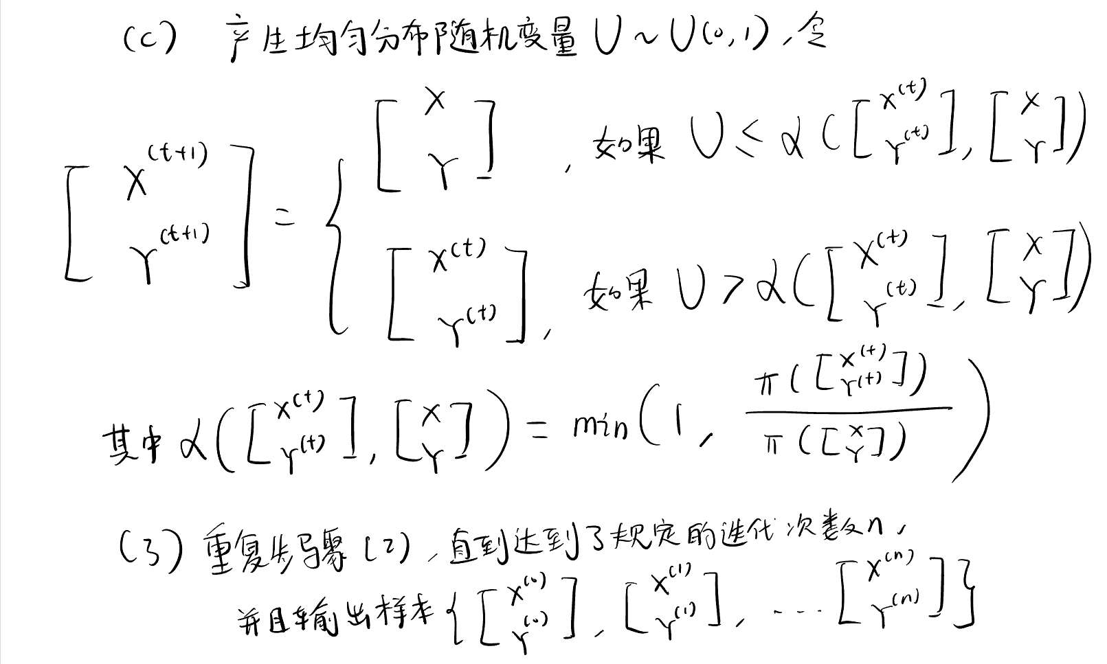
初始化样本
Text Only
样本的初始值为: [0 0]
设定迭代次数
迭代产生样本
Python
for t in tqdm(range(iteration)):
    # 生成正态分布随机数
    vector_e1_e2_ = np.random.normal(0, 1, 2)
    # 将上一步生成的随机数加到 x 和 y 上
    vector_x_y_ = vector_x_y + vector_e1_e2_
    # 计算接受率
    ratio = two_dimensional_gaussian(vector_x_y_, mu, sigma) / two_dimensional_gaussian(
        vector_x_y, mu, sigma
    )
    alpha = min(1, ratio)
    # 生成一个随机数 u,它来自均匀分布
    u = np.random.uniform(0, 1)
    # 如果接受率大于 u,则接受,即更新 x 和 y 的值
    if alpha > u:
        vector_x_y = vector_x_y_
        accept += 1
    # 保存样本
    # 第一次迭代时,初始化样本
    if t == 0:
        samples_random_walk = vector_x_y.copy()
    # 后续迭代时,将样本添加到样本集中
    else:
        samples_random_walk = np.vstack((samples_random_walk, vector_x_y))
# 计算接受率
accept_rate = accept / iteration
print("接受率:{:.2%}".format(accept_rate))
Text Only
100%|██████████| 100000/100000 [00:24<00:00, 4091.07it/s]

接受率:45.51%
Text Only
array([[ 0.        ,  0.        ],
       [ 0.        ,  0.        ],
       [ 0.        ,  0.        ],
       ...,
       [-0.71973486, -1.23049515],
       [-0.71973486, -1.23049515],
       [ 0.33205658, -0.79309342]])
收敛性诊断——依据各分量的累计均值
Text Only
array([[   0.        ,    0.        ],
       [   0.        ,    0.        ],
       [   0.        ,    0.        ],
       ...,
       [1019.11864357, 1477.36299153],
       [1018.39890871, 1476.13249638],
       [1018.73096529, 1475.33940296]])
Text Only
array([[     1],
       [     2],
       [     3],
       ...,
       [ 99998],
       [ 99999],
       [100000]])
Python
fig = plt.figure(figsize=(10, 6))
plt.plot(cummean, label=["x", "y"])
# 绘制辅助线,纵坐标为 0
plt.axhline(0, color="black", linestyle="--")
plt.legend()
plt.show()
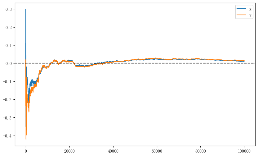
可以看到,当迭代次数达到 50000 时,\(x\)和\(y\)的累计均值都已经趋于一条直线,但还没有非常接近 0。
独立性抽样
初始化样本
Python
x = 0
y = 0
vector_x_y = np.array([x, y])
# 构造二维独立标准正态分布的理论分布
g = multivariate_normal(mean=np.zeros(2), cov=np.eye(2))
设定迭代次数
迭代产生样本
Python
for t in tqdm(range(iteration)):
    # 生成正态分布随机数
    vector_e1_e2_ = np.random.normal(0, 1, 2)
    # 将随机数直接赋值到 x 和 y 上
    vector_x_y_ = vector_e1_e2_
    # 计算接受率
    ratio = (two_dimensional_gaussian(vector_x_y_, mu, sigma) * g.pdf(vector_x_y)) / (
        two_dimensional_gaussian(vector_x_y, mu, sigma) * g.pdf(vector_x_y_)
    )
    alpha = min(1, ratio)
    # 生成一个随机数 u,它来自均匀分布
    u = np.random.uniform(0, 1)
    # 如果接受率大于 u,则接受,即更新 x 和 y 的值
    if alpha > u:
        vector_x_y = vector_x_y_
        accept += 1
    # 保存样本
    # 第一次迭代时,初始化样本
    if t == 0:
        samples_independent = vector_x_y.copy()
    # 后续迭代时,将样本添加到样本集中
    else:
        samples_independent = np.vstack((samples_independent, vector_x_y))
# 计算接受率
accept_rate = accept / iteration
print("接受率:{:.2%}".format(accept_rate))
Text Only
100%|██████████| 100000/100000 [00:27<00:00, 3602.83it/s]

接受率:58.18%
收敛性诊断——依据各分量的累计均值
Text Only
array([[   0.        ,    0.        ],
       [  -0.98714667,   -0.81647526],
       [  -1.97429335,   -1.63295051],
       ...,
       [-380.02483172, -540.44083572],
       [-379.2919882 , -540.70237326],
       [-380.33205906, -541.43726736]])
Python
fig = plt.figure(figsize=(10, 6))
plt.plot(cummean, label=["x", "y"])
# 绘制辅助线,纵坐标为 0
plt.axhline(0, color="black", linestyle="--")
plt.legend()
plt.show()
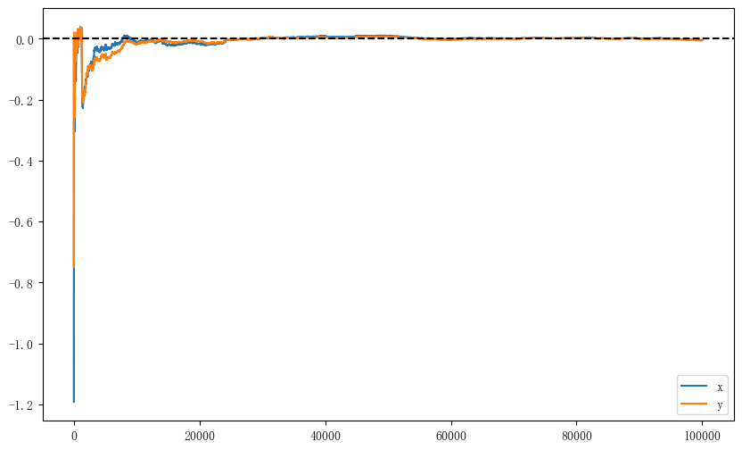
可以看到,当迭代次数达到 30000 时,\(x\)和\(y\)的累计均值都已经趋于 0,说明样本已经收敛。
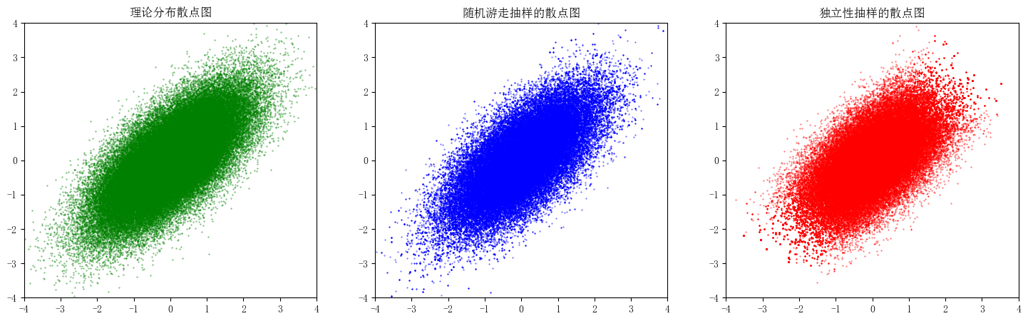
绘制样本的散点图
Python
fig = plt.figure(figsize=(18, 5))

# 绘制理论分布的散点图
ax1 = fig.add_subplot(131)
# 生成理论分布的样本
theoretical_sample = var.rvs(100000)
ax1.scatter(theoretical_sample[:, 0], theoretical_sample[:, 1], s=0.1, c="g")
# 标题
ax1.set_title("理论分布散点图")

# 绘制随机游走抽样的样本散点图
ax2 = fig.add_subplot(132)
ax2.scatter(samples_random_walk[:, 0], samples_random_walk[:, 1], s=0.1, c="b")
# 标题
ax2.set_title("随机游走抽样的散点图")

# 绘制独立性抽样的样本散点图
ax3 = fig.add_subplot(133)
ax3.scatter(samples_independent[:, 0], samples_independent[:, 1], s=0.1, c="r")
# 标题
ax3.set_title("独立性抽样的散点图")

# 统一坐标轴范围
for ax in fig.axes:
    ax.set_xlim(-4, 4)
    ax.set_ylim(-4, 4)

plt.show()
Python
# 将三种抽样的散点图放在一起
fig = plt.figure(figsize=(6, 6))
plt.scatter(
    theoretical_sample[:, 0], theoretical_sample[:, 1], s=0.1, c="g", label="理论分布"
)
plt.scatter(
    samples_random_walk[:, 0], samples_random_walk[:, 1], s=0.1, c="b", label="随机游走抽样"
)
plt.scatter(
    samples_independent[:, 0], samples_independent[:, 1], s=0.1, c="r", label="独立性抽样"
)
plt.legend()
plt.show()
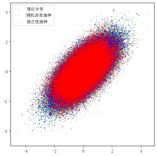
比较两种算法的表现
- 随机游走算法的接受率为 45% 左右,独立性抽样的接受率为 55% 左右。
- 随机游走算法的累计均值在前期震荡幅度较大,收敛所需的迭代次数也更多。
- 独立性抽样的累计均值在前期震荡幅度较小,收敛所需的迭代次数也更少,只需迭代 30000 次左右,累计均值就收敛到 0 了。
- 两种算法的样本散点图基本一致,但独立性抽样的样本散点图更加集中,即尾部的样本更少。