K 折、随机和时间序列交叉验证的 Python 实现¶

相比 K 折、随机交叉验证方法，时序交叉验证方法不会用到未来信息预测历史结果，在测试集上的表现更稳健。时序交叉验证在时序数据上可以缓解过拟合问题，且训练耗时更少。

png

本文使用论坛文本数据（每日 25 条新闻标题）对道琼斯工业指数的涨跌方向进行分类预测。（数据来源：Kaggle Dataset）在信噪比极低的金融数据中，我们不期望预测效果有多么优秀。因此本文将重心放在多种交叉验证方法的实现与结果对比上。

我们发现 Shuffle 交叉验证在验证集上表现虽然优秀，但用到了很多未来信息预测历史结果，这是一种“作弊”行为，在现实中也是无法做到的。

在样本不满足独立同分布假设的时间序列数据上（如金融数据、医疗监测数据、销量数据等），更推荐使用时序交叉验证缓解过拟合问题，且训练时间开销更少。

特征工程代码片段¶

词频统计¶

Python

# 词频统计
cnt_vectorizer = CountVectorizer(min_df=0.05)
cnt_train = cnt_vectorizer.fit_transform(train_headlines)
cnt_test = cnt_vectorizer.transform(test_headlines)
print(cnt_train.shape)
ev(cnt_train, cnt_test, cnt_vectorizer.get_feature_names())

TF-IDF¶

Python

# TF-IDF
tfidf_vectorizer = TfidfVectorizer(stop_words="english")
tfidf_train = tfidf_vectorizer.fit_transform(train_headlines)
tfidf_test = tfidf_vectorizer.transform(test_headlines)
print(tfidf_train.shape)
ev(tfidf_train, tfidf_test, tfidf_vectorizer.get_feature_names())

2-gram TF-IDF¶

Python

# TF-IDF: 2-gram
gram_vectorizer = TfidfVectorizer(min_df=0.03, ngram_range=(2, 2))
gram_train = gram_vectorizer.fit_transform(train_headlines)
gram_test = gram_vectorizer.transform(test_headlines)
gram_train.shape
ev(gram_train, gram_test, gram_vectorizer.get_feature_names())

交叉验证——以 XGBoost 为例¶

K 折和 Shuffle 交叉验证在验证集上的表现比在测试集上的表现优秀很多。我们认为可能是因为它们在训练集中泄露了未来信息。举例来说，如果我们在今天观察到输入信息是“Market Expansion”，并且股价是上涨的，此时如果我们要回头预测上个月的标签，发现上个月的输入信息也是“Market Expansion”，我们很可能会完美地预测股价上涨，并且预测正确。但是，在真实的环境下，我们在预测 11 月份标签的时候，只能看到 11 月 25 日及之前的情况，这时我们不知道“Market Expansion”对应的是什么标签，因此很可能预测不准确。

为了避免未来信息泄露，我们需要保证训练集在验证集之前。同时，交叉验证的思想是尽量多利用数据，所以我们采用时序交叉验证的办法。许多文献也表明，时序交叉验证在应对时序数据集上优于传统的交叉验证方法。

Python

from sklearn.model_selection import KFold, ShuffleSplit, TimeSeriesSplit
import xgboost as xgb
from sklearn.model_selection import GridSearchCV, RandomizedSearchCV
import numpy as np
from tqdm import tqdm
import matplotlib.pyplot as plt
from matplotlib.patches import Patch
from matplotlib.ticker import PercentFormatter

交叉验证的数据¶

Python

# 定义交叉验证所需的训练集、验证集和测试集
X_train_and_validation_for_cv = gram_train.toarray()
y_train_and_validation_for_cv = train["Label"].values
X_test_for_cv = gram_test.toarray()
y_test_for_cv = test["Label"].values

定义交叉验证划分方法的实例¶

Python

# 定义 n_splits
n_splits = 5
# 定义交叉验证的实例
split_kfold = KFold(n_splits=n_splits)
split_shuffle = ShuffleSplit(n_splits=n_splits, test_size=1 / n_splits, random_state=0)
split_ts = TimeSeriesSplit(n_splits=n_splits)

定义函数，绘制不同交叉验证方法下，训练集和验证集的分布情况¶

Python

def plot_cv_indices(split_method, X, ax, n_splits, lw=10):
    """
    绘制交叉验证的训练集和验证集的分布情况

    """

    # 生成交叉验证中训练集和验证集的索引
    for ii, (tr, tt) in enumerate(split_method.split(X=X)):
        # 填充训练集和验证集的索引
        indices = np.array([np.nan] * len(X))
        indices[tt] = 1
        indices[tr] = 0
        # 绘制每一个交叉验证的训练集和验证集的分布情况
        ax.scatter(
            range(len(indices)),
            [ii + 0.5] * len(indices),
            c=indices,
            marker="_",
            lw=lw,
            cmap=plt.cm.coolwarm,
            vmin=-0.2,
            vmax=1.2,
        )
    yticklabels = list(range(1, n_splits + 1))
    ax.set(
        yticks=np.arange(n_splits) + 0.5,
        yticklabels=yticklabels,
        xlabel="Index",
        ylabel="CV iteration",
        ylim=[n_splits, -0.2],
        xlim=[0, X_train_and_validation_for_cv.shape[0]],
    )
    ax.set_title("{}".format(type(split_method).__name__), fontsize=15)
    return ax

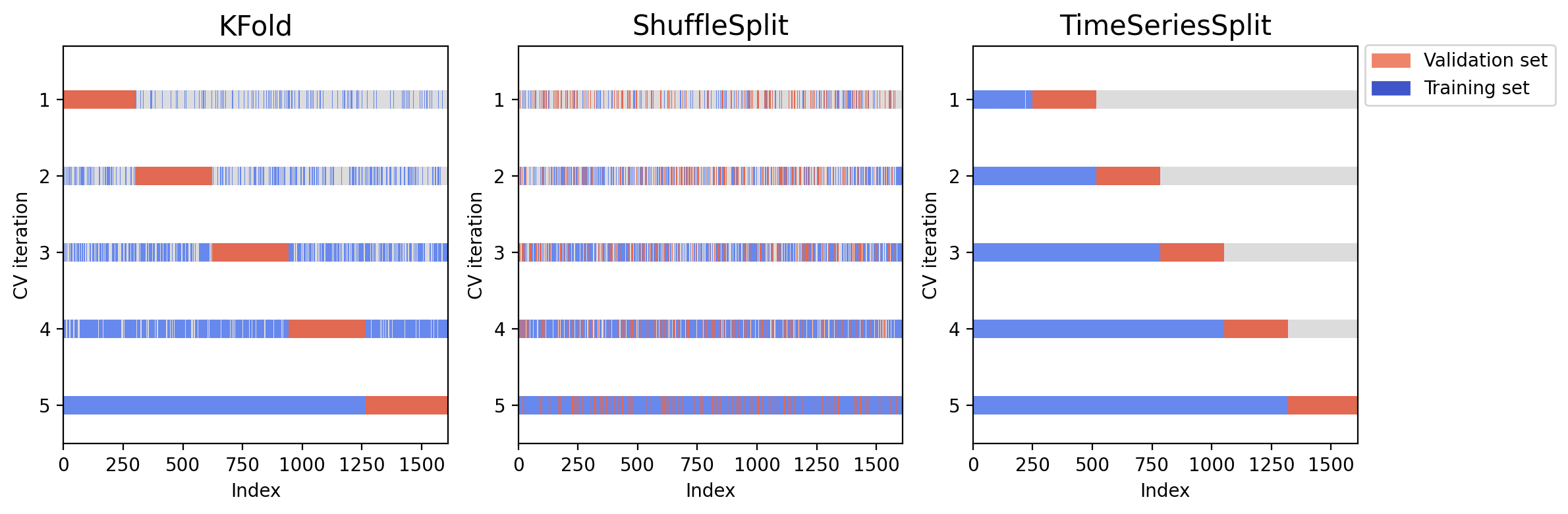
绘制不同交叉验证方法下，训练集和验证集的分布情况¶

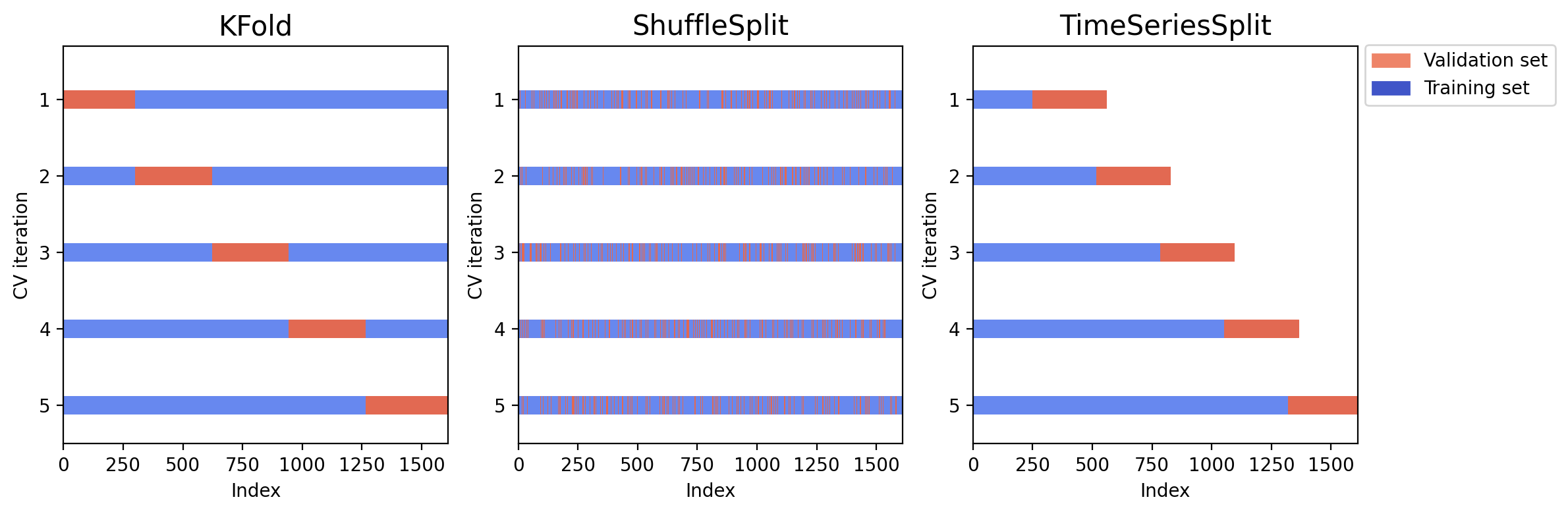
这幅图展示了三种交叉验证方法的划分结果。蓝色是训练集，红色是验证集。可以看到，K 折和 Shuffle 交叉验证都使用了未来信息来预测历史结果，而时序交叉验证很好地保证了训练集和验证集的先后顺序。

Python

fig = plt.figure(figsize=(12, 4), dpi=200)
for i, split_method in enumerate([split_kfold, split_shuffle, split_ts]):
    ax = fig.add_subplot(1, 3, 1 + i)
    plot_cv_indices(split_method, X_train_and_validation_for_cv, ax, n_splits)
# 绘制图例
ax.legend(
    [Patch(color=plt.cm.coolwarm(0.8)), Patch(color=plt.cm.coolwarm(0.02))],
    ["Validation set", "Training set"],
    loc=(1.02, 0.85),
)
plt.tight_layout()
plt.show()

png

定义函数，汇总不同交叉验证方法下的最优参数¶

Python

def get_best_params(cv_results):
    # 将各个交叉验证方法寻找到的最佳参数进行汇总
    best_params = pd.DataFrame.from_dict(
        {method: cv_results[method]["Best_Params"] for method in cv_results.keys()},
        orient="index",
    )
    # 删去 eval_metric 参数
    best_params.drop("eval_metric", axis=1, inplace=True)
    return best_params

定义函数，绘制不同交叉验证方法下的平均验证集准确率和测试集准确率¶

Python

def plot_mean_validation_accuracy_and_test_accuracy(cv_results):
    # 绘制不同交叉验证方法下的平均验证集准确率
    fig = plt.figure(figsize=(6, 4), dpi=200)
    ax = fig.add_subplot(1, 1, 1)
    ax.bar(
        x=np.arange(len(cv_results)),
        height=[
            cv_results[method]["Mean_Validation_Accuracy"] for method in cv_results
        ],
        tick_label=[method for method in cv_results],
        color="steelblue",
        alpha=0.8,
        width=0.4,
        label="Mean Validation Accuracy",
    )
    # 在柱状图上方添加数字标签
    for x, y in enumerate(
        [cv_results[method]["Mean_Validation_Accuracy"] for method in cv_results]
    ):
        plt.text(x, y + 0.001, "{:.2%}".format(y), ha="center", va="bottom")
    # 绘制不同交叉验证方法下的测试集准确率
    ax.bar(
        x=np.arange(0.4, len(cv_results)),
        height=[cv_results[method]["Test_Accuracy"] for method in cv_results],
        tick_label=[method for method in cv_results],
        color="indianred",
        alpha=0.8,
        width=0.4,
        label="Test Accuracy",
    )
    # 在柱状图上方添加数字标签
    for x, y in enumerate(
        [cv_results[method]["Test_Accuracy"] for method in cv_results]
    ):
        plt.text(x + 0.4, y + 0.001, "{:.2%}".format(y), ha="center", va="bottom")
    # x 轴的刻度
    ax.set_xticks(np.arange(0.2, len(cv_results)))
    ax.set_xticklabels([method for method in cv_results])
    ax.set_ylim([0.5, 0.58])
    # ylabel 以百分数的形式显示
    ax.yaxis.set_major_formatter(PercentFormatter(1.0, decimals=0))
    ax.set_ylabel("Accuracy")
    ax.legend(fontsize=8)
    plt.show()

时序交叉验证的实现方法¶

第一种方法是向 cross_validation 方法中对folds参数直接传入一个Split实例。第二种方法是传入一个元组，这个元组包含了自定义的训练集索引和验证集索引，可以高度地定制任意训练集和验证集地划分方法。

详细的代码可以参考这篇帖子。

网格搜索¶

网格搜索面临维数灾难，耗时较长，因此只尝试少量参数组合。

Python

# 定义字典，用于存储不同交叉验证方法的结果
cv_results_grid = {}
# 定义网格搜索的参数
param_grid = {
    "eta": [0.001, 0.01],
    "gamma": [1, 0.1],
    "max_depth": [2, 3],
    "min_child_weight": [2, 3],
    "eval_metric": ["logloss"],
}
for split_method in tqdm([split_kfold, split_shuffle, split_ts]):
    cv_results_grid[type(split_method).__name__] = {
        "Best_Params": None,
        "Mean_Validation_Accuracy": None,
        "Test_Accuracy": None,
    }
    # 定义网格搜索的实例
    grid_search = GridSearchCV(
        estimator=xgb.XGBClassifier(tree_method="gpu_hist"),
        param_grid=param_grid,
        cv=split_method,
        scoring="accuracy",
        n_jobs=-1,
        verbose=1,
    )
    # 进行网格搜索
    grid_search.fit(X_train_and_validation_for_cv, y_train_and_validation_for_cv)
    # 记录最佳参数
    cv_results_grid[type(split_method).__name__][
        "Best_Params"
    ] = grid_search.best_params_
    # 记录最佳参数下的平均验证集准确率
    cv_results_grid[type(split_method).__name__][
        "Mean_Validation_Accuracy"
    ] = grid_search.best_score_
    # 记录最佳参数下的测试集准确率
    cv_results_grid[type(split_method).__name__]["Test_Accuracy"] = grid_search.score(
        X_test_for_cv, y_test_for_cv
    )

Text Only

Fitting 5 folds for each of 16 candidates, totalling 80 fits

100%|██████████| 3/3 [01:00<00:00, 20.05s/it]

Python

get_best_params(cv_results_grid)

	eta	gamma	max_depth	min_child_weight
KFold	0.001	1.0	3	2
ShuffleSplit	0.001	1.0	2
TimeSeriesSplit	0.010	0.1	2

Python

plot_mean_validation_accuracy_and_test_accuracy(cv_results_grid)

png

随机搜索¶

Python

# 定义字典，用于存储不同交叉验证方法的结果
cv_results_random = {}
# 定义随机搜索的参数
param_grid = {
    "eta": [0.005, 0.01, 0.015],
    "gamma": [1, 0.1, 0.01],
    "max_depth": [2, 3, 4, 5],
    "min_child_weight": [2, 3, 4, 5],
    "eval_metric": ["logloss"],
}
for split_method in tqdm([split_kfold, split_shuffle, split_ts]):
    cv_results_random[type(split_method).__name__] = {
        "Best_Params": None,
        "Mean_Validation_Accuracy": None,
        "Test_Accuracy": None,
    }
    # 定义随机搜索的实例
    rondom_search = RandomizedSearchCV(
        estimator=xgb.XGBClassifier(tree_method="gpu_hist"),
        param_distributions=param_grid,
        n_iter=20,
        cv=split_method,
        scoring="accuracy",
        n_jobs=-1,
        verbose=1,
        random_state=0,
    )
    # 进行随机搜索
    rondom_search.fit(X_train_and_validation_for_cv, y_train_and_validation_for_cv)
    # 记录最佳参数
    cv_results_random[type(split_method).__name__][
        "Best_Params"
    ] = rondom_search.best_params_
    # 记录最佳参数下的平均验证集准确率
    cv_results_random[type(split_method).__name__][
        "Mean_Validation_Accuracy"
    ] = rondom_search.best_score_
    # 记录最佳参数下的测试集准确率
    cv_results_random[type(split_method).__name__][
        "Test_Accuracy"
    ] = rondom_search.score(X_test_for_cv, y_test_for_cv)

Text Only

Fitting 5 folds for each of 20 candidates, totalling 100 fits

100%|██████████| 3/3 [01:29<00:00, 29.67s/it]

从众多参数组合中随机选出 20 个，再从这 20 个参数组合中选出在验证集上平均预测准确率最高的。

Python

get_best_params(cv_results_random)

	min_child_weight	max_depth	gamma	eta
KFold	5	4	1.0	0.010
ShuffleSplit	2	0.1	0.005
TimeSeriesSplit	5	4	1.0	0.010

Python

plot_mean_validation_accuracy_and_test_accuracy(cv_results_random)

png

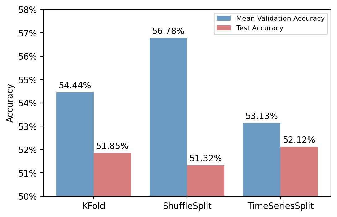
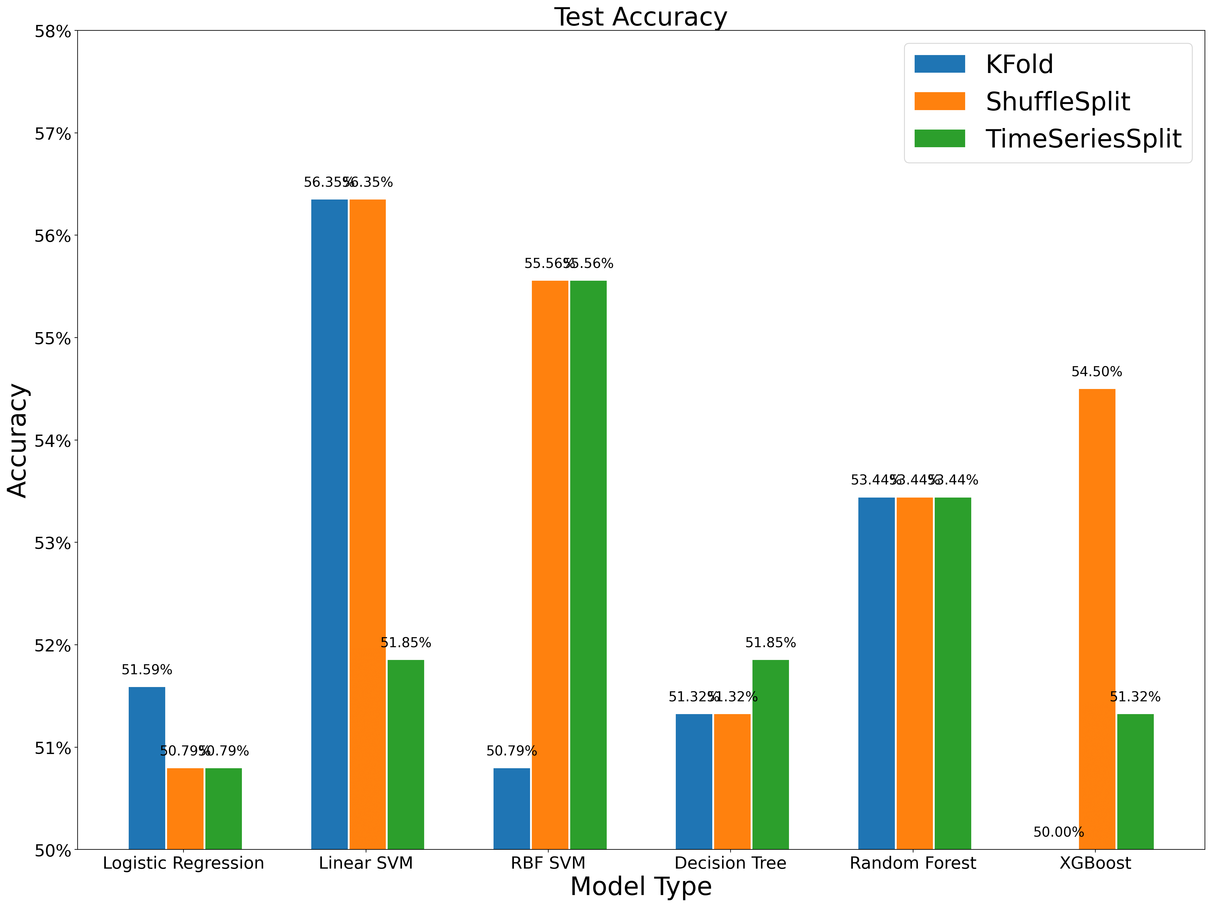
可以看到，ShuffleSplit 方法存在明显的过拟合问题，其在交叉验证时的验证集上表现非常好，但在测试集上表现最差。TimeSeriesSplit 方法虽然在交叉验证时表现较差，但在测试集上表现最好。

交叉验证——对比多种模型¶

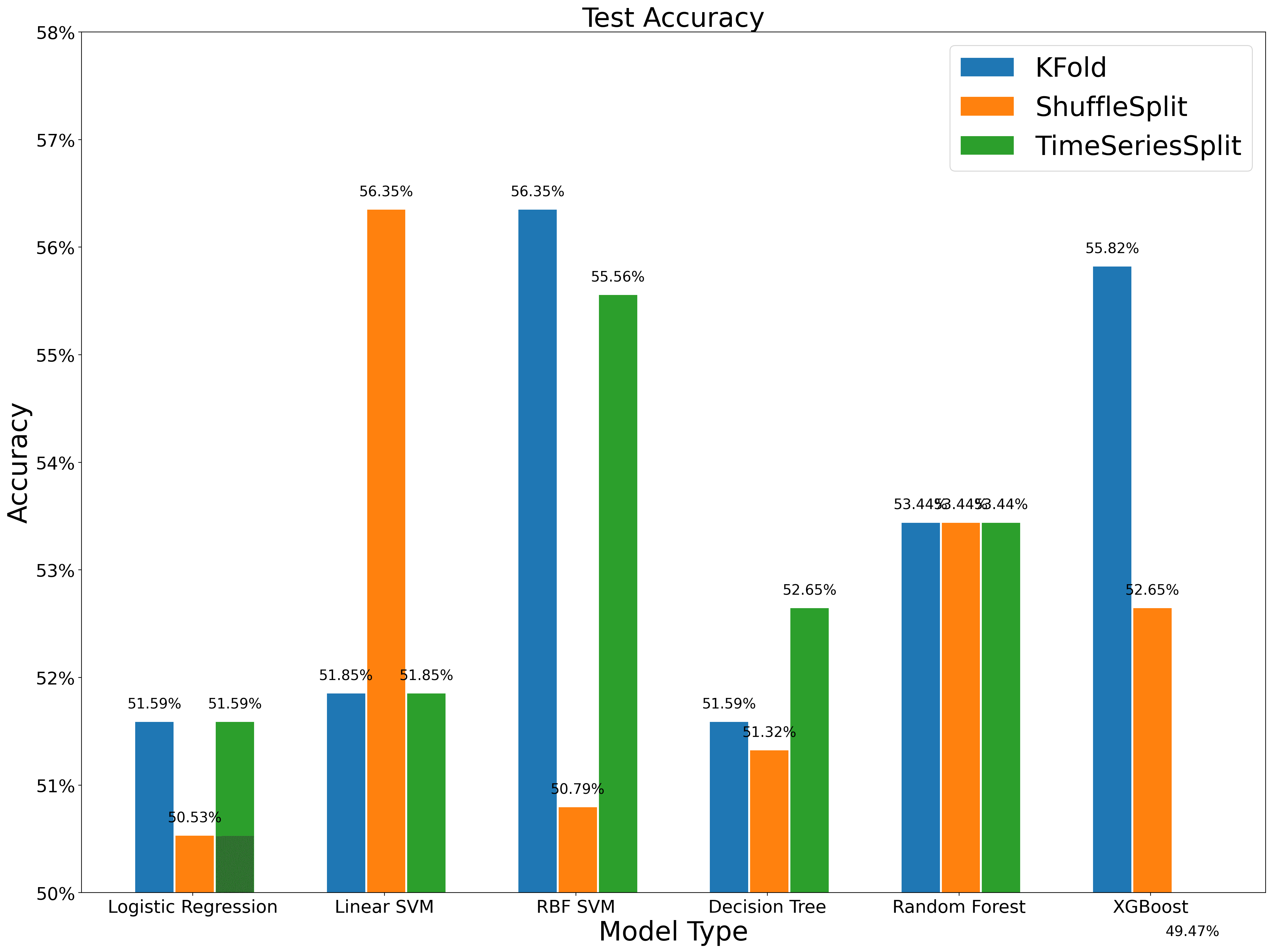
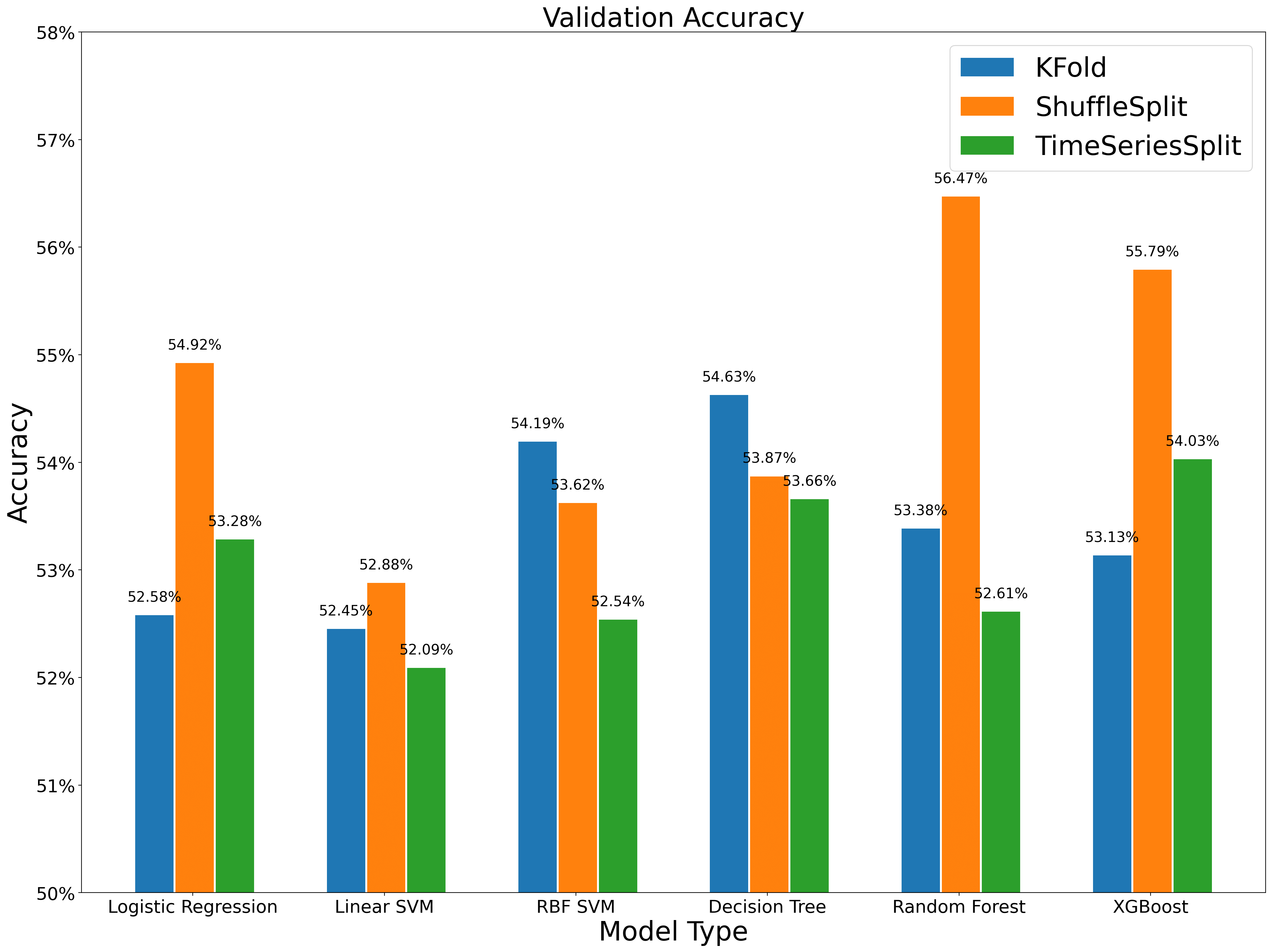
在多个模型上进行训练，发现 Shuffle 方法在验证集上总是表现最好的那个，但在测试集上的表现并不稳定。尤其是复杂的高斯核 SVM 和 XGBoost 模型，我们推测是因为复杂的模型对超参数更加敏感。

Python

def cv_grid_one(model):
    # 定义字典，用于存储不同交叉验证方法的结果
    cv_results_grid = {}
    # 定义网格搜索的参数
    param_grid = {
        "eta": [0.001, 0.01],
        "gamma": [1, 0.1],
        "max_depth": [2, 3],
        "min_child_weight": [2, 3],
        "eval_metric": ["logloss"],
    }
    for split_method in tqdm([split_kfold, split_shuffle, split_ts]):
        cv_results_grid[type(split_method).__name__] = {
            "Best_Params": None,
            "Mean_Validation_Accuracy": None,
            "Test_Accuracy": None,
        }
        # 定义网格搜索的实例
        grid_search = GridSearchCV(
            estimator=model,
            param_grid=param_grid,
            cv=split_method,
            scoring="accuracy",
            n_jobs=-1,
            verbose=1,
        )
        # 进行网格搜索
        t1 = time.time()
        grid_search.fit(X_train_and_validation_for_cv, y_train_and_validation_for_cv)
        t2 = time.time()
        # 记录最佳参数
        cv_results_grid[type(split_method).__name__][
            "Best_Params"
        ] = grid_search.best_params_
        # 记录最佳参数下的平均验证集准确率
        cv_results_grid[type(split_method).__name__][
            "Mean_Validation_Accuracy"
        ] = grid_search.best_score_
        # 记录最佳参数下的测试集准确率
        cv_results_grid[type(split_method).__name__][
            "Test_Accuracy"
        ] = grid_search.score(X_test_for_cv, y_test_for_cv)
        cv_results_grid[type(split_method).__name__]["time"] = t2 - t1
        cv_results_grid[type(split_method).__name__][
            "best_estimator"
        ] = grid_search.best_estimator_
    return cv_results_grid

Python

from scipy.stats import randint
from scipy.stats import uniform


def cv_random_one(model):
    # 定义字典，用于存储不同交叉验证方法的结果
    cv_results_random = {}
    # 定义随机搜索的参数
    if model == xgb_model:
        param_random = {
            "eta": [0.005, 0.01, 0.015],
            "gamma": [1, 0.1, 0.01],
            "max_depth": [2, 3, 4, 5],
            "min_child_weight": [2, 3, 4, 5],
            "eval_metric": ["logloss"],
        }
    if model == linearsvm_model or model == gssvm_model:
        param_random = {"C": [1, 10, 100, 1000], "gamma": [1, 0.1, 0.01, 0.001]}

    if model == RF_model:
        param_random = {
            "n_estimators": randint(low=1, high=200),
            "max_features": randint(low=7, high=9),
        }

    if model == tree_model:
        param_random = {"max_depth": [1, 2, 3, 4, 5, 6, 7, None]}

    if model == LR_model:
        param_random = {"C": uniform(loc=0, scale=4), "penalty": ["l2", "l1"]}

    for split_method in tqdm([split_kfold, split_shuffle, split_ts]):
        cv_results_random[type(split_method).__name__] = {
            "Best_Params": None,
            "Mean_Validation_Accuracy": None,
            "Test_Accuracy": None,
        }
        # 定义随机搜索的实例
        rondom_search = RandomizedSearchCV(
            estimator=model,
            param_distributions=param_random,
            n_iter=20,
            cv=split_method,
            scoring="accuracy",
            n_jobs=-1,
            verbose=1,
            random_state=0,
        )
        # 进行随机搜索
        t1 = time.time()
        rondom_search.fit(X_train_and_validation_for_cv, y_train_and_validation_for_cv)
        t2 = time.time()
        # 记录最佳参数下的平均验证集准确率
        cv_results_random[type(split_method).__name__][
            "Mean_Validation_Accuracy"
        ] = rondom_search.best_score_
        # 记录最佳参数下的测试集准确率
        cv_results_random[type(split_method).__name__][
            "Test_Accuracy"
        ] = rondom_search.score(X_test_for_cv, y_test_for_cv)
        # 时间
        cv_results_random[type(split_method).__name__]["time"] = t2 - t1
        cv_results_random[type(split_method).__name__][
            "best_estimator"
        ] = rondom_search.best_estimator_
    return cv_results_random

Python

import matplotlib
import matplotlib.pyplot as plt
import numpy as np


def autolabel(rects):
    """在* rects *中的每个柱状条上方附加一个文本标签，显示其高度"""
    for rect in rects:
        height = rect.get_height()
        ax.annotate(
            "{}".format(height),
            xy=(rect.get_x() + rect.get_width() / 2, height),
            xytext=(0, 3),  # 3 点垂直偏移
            textcoords="offset points",
            ha="center",
            va="bottom",
        )


def plot_compare(a, b, c, title):
    fig = plt.figure(figsize=(20, 15), dpi=200)
    ax = fig.add_subplot(1, 1, 1)
    # plt.rcParams['font.sans-serif']=['SimHei'] # 解决中文乱码
    labels = [
        "Logistic Regression",
        "Linear SVM",
        "RBF SVM",
        "Decision Tree",
        "Random Forest",
        "XGBoost",
    ]
    x = np.arange(len(labels))  # 标签位置
    width = 0.2  # 柱状图的宽度，可以根据自己的需求和审美来改
    rects1 = ax.bar(x - width, a, width, label="KFold")
    rects2 = ax.bar(x + 0.01, b, width, label="ShuffleSplit")
    rects3 = ax.bar(x + 0.02 + width, c, width, label="TimeSeriesSplit")
    # 为 y 轴、标题和 x 轴等添加一些文本。

    # 在柱状图上方添加数字标签
    if title != "Time":
        for m, y in enumerate(a):
            plt.text(
                m - width,
                y + 0.001,
                "{:.2%}".format(y),
                ha="center",
                va="bottom",
                fontsize=16,
            )
        for m, y in enumerate(b):
            plt.text(
                m + 0.01,
                y + 0.001,
                "{:.2%}".format(y),
                ha="center",
                va="bottom",
                fontsize=16,
            )
        for m, y in enumerate(c):
            plt.text(
                m + 0.02 + width,
                y + 0.001,
                "{:.2%}".format(y),
                ha="center",
                va="bottom",
                fontsize=16,
            )
        ax.set_ylim([0.5, 0.58])
        ax.yaxis.set_major_formatter(PercentFormatter(1.0, decimals=0))
        ax.set_ylabel("Accuracy", fontsize=30)
        ax.set_xlabel("Model Type", fontsize=30)
    if title == "Time":
        for m, y in enumerate(a):
            plt.text(
                m - width,
                y + 0.001,
                "{:.2f}".format(y),
                ha="center",
                va="bottom",
                fontsize=16,
            )
        for m, y in enumerate(b):
            plt.text(
                m + 0.01,
                y + 0.001,
                "{:.2f}".format(y),
                ha="center",
                va="bottom",
                fontsize=16,
            )
        for m, y in enumerate(c):
            plt.text(
                m + 0.02 + width,
                y + 0.001,
                "{:.2f}".format(y),
                ha="center",
                va="bottom",
                fontsize=16,
            )
        ax.set_ylabel("Time", fontsize=16)
        ax.set_xlabel("Model Type", fontsize=16)
    ax.set_title(title, fontsize=30)
    ax.set_xticks(x)
    ax.set_xticklabels(labels, fontsize=20)
    ax.tick_params(labelsize=20)
    ax.legend(fontsize=30)
    # ylabel 以百分数的形式显示

    autolabel(rects1)
    autolabel(rects2)
    autolabel(rects3)

    fig.tight_layout()
    plt.show()

Python

a_valid = list()
b_valid = list()
c_valid = list()
a_test = list()
b_test = list()
c_test = list()
a_time = list()
b_time = list()
c_time = list()
for model in [xgb_model, linearsvm_model, gssvm_model, tree_model, LR_model, RF_model]:
    k = cv_random_one(model)

    a_valid.append(k["KFold"]["Mean_Validation_Accuracy"])
    b_valid.append(k["ShuffleSplit"]["Mean_Validation_Accuracy"])
    c_valid.append(k["TimeSeriesSplit"]["Mean_Validation_Accuracy"])
    a_test.append(k["KFold"]["Test_Accuracy"])
    b_test.append(k["ShuffleSplit"]["Test_Accuracy"])
    c_test.append(k["TimeSeriesSplit"]["Test_Accuracy"])
    a_time.append(k["KFold"]["time"])
    b_time.append(k["ShuffleSplit"]["time"])
    c_time.append(k["TimeSeriesSplit"]["time"])
plot_compare(a_valid, b_valid, c_valid, "Validation Accuracy")
plot_compare(a_test, b_test, c_test, "Test Accuracy")
plot_compare(a_time, b_time, c_time, "Time")

png

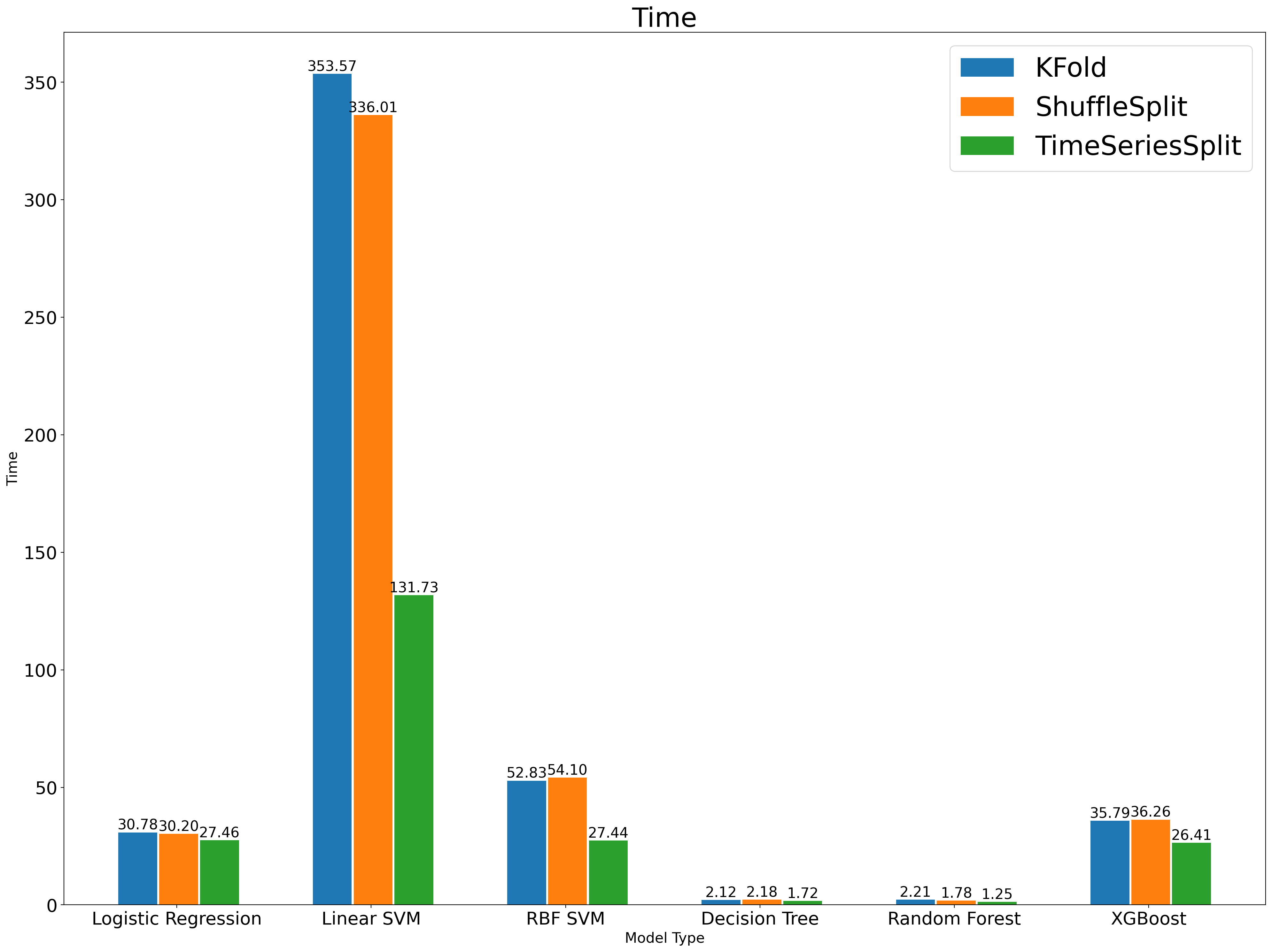
最后我们比较了三种方法的训练时间，可以看到时序交叉验证的耗时基本是其他两种方法的一半，这本质上是因为它整体上只用到了一半的训练数据。这也给了我们一个启发：训练集的样本量也是影响拟合程度的因素，如果控制住它，结论会不会仍然成立呢？

控制训练集样本量¶

时序交叉验证带来的预测效果的提升，究竟是

保留了样本的时序信息；
还是因为时序交叉验证使用更少（接近一半）的样本量。

定义颜色 Colormap，将未被选为训练集的样本描述为白色。

将 K 折和 Shuffle 的训练集样本量减少到和时序交叉验证相同。图中的蓝色仍然是训练集，红色仍然是验证集，但有一部分的白色是被我们剔除的训练集，这样我们就能够控制三种方法的训练集样本量。

Python

from matplotlib.colors import LinearSegmentedColormap

# Create a new colormap that goes from blue to white to red
my_colormap = LinearSegmentedColormap.from_list(
    "my_colormap", [(0, "blue"), (0.5, "white"), (1, "red")]
)

Python

def split_less_sample(split_method, X):
    in_and_out_list = []
    i = 1
    for train_index, test_index in split_method.split(X=X):
        train_index = list(train_index)
        test_index = list(test_index)
        # Randomly shuffle the list
        random.shuffle(train_index)
        # Delete some items from the list
        if i != n_splits:  # 若没到最后一轮，则需要减少传统交叉验证的训练集样本量
            train_index = train_index[: i * (len(X)) // (n_splits + 1)]
        i += 1
        # Sort the list
        train_index.sort()
        in_and_out = (train_index, test_index)
        in_and_out_list.append(in_and_out)
    return in_and_out_list

Python

def plot_cv_indices_less_sample(split_method, X, ax, n_splits, lw=10):
    """
    绘制交叉验证的训练集和验证集的分布情况，并且训练集的样本量保证与时序交叉验证的训练集样本量相同

    """

    in_and_out_list = split_less_sample(split_method, X)
    #     print(in_and_out_list)
    # 生成交叉验证中训练集和验证集的索引
    for ii, (tr, tt) in enumerate(in_and_out_list):
        # 填充训练集和验证集的索引
        indices = np.array([np.nan] * len(X))
        indices[tt] = 1
        indices[tr] = 0
        indices[np.where(np.isnan(indices))] = 0.5
        #         print(indices)
        # 绘制每一个交叉验证的训练集和验证集的分布情况
        ax.scatter(
            range(len(indices)),
            [ii + 0.5] * len(indices),
            c=indices,
            marker="_",
            lw=lw,
            cmap=plt.cm.coolwarm,
            vmin=-0.2,
            vmax=1.2,
        )
    yticklabels = list(range(1, n_splits + 1))
    ax.set(
        yticks=np.arange(n_splits) + 0.5,
        yticklabels=yticklabels,
        xlabel="Index",
        ylabel="CV iteration",
        ylim=[n_splits, -0.2],
        xlim=[0, X_train_and_validation_for_cv.shape[0]],
    )
    ax.set_title("{}".format(type(split_method).__name__), fontsize=15)
    return ax

Python

fig = plt.figure(figsize=(12, 4), dpi=200)
split_kfold = KFold(n_splits=n_splits)
split_shuffle = ShuffleSplit(n_splits=n_splits, test_size=1 / n_splits, random_state=0)
split_ts = TimeSeriesSplit(n_splits=n_splits)
for i, split_method in enumerate([split_kfold, split_shuffle, split_ts]):
    ax = fig.add_subplot(1, 3, 1 + i)
    plot_cv_indices_less_sample(
        split_method, X_train_and_validation_for_cv, ax, n_splits
    )
# 绘制图例
ax.legend(
    [Patch(color=plt.cm.coolwarm(0.8)), Patch(color=plt.cm.coolwarm(0.02))],
    ["Validation set", "Training set"],
    loc=(1.02, 0.85),
)
plt.tight_layout()
plt.show()

png

在相同训练集样本量的情况下，比较各模型的优劣¶

Python

def cv_random_one_less_sample(model):
    # 定义字典，用于存储不同交叉验证方法的结果
    cv_results_random = {}
    # 定义随机搜索的参数
    if model == xgb_model:
        param_random = {
            "eta": [0.005, 0.01, 0.015],
            "gamma": [1, 0.1, 0.01],
            "max_depth": [2, 3, 4, 5],
            "min_child_weight": [2, 3, 4, 5],
            "eval_metric": ["logloss"],
        }
    if model == linearsvm_model or model == gssvm_model:
        param_random = {"C": [1, 10, 100, 1000], "gamma": [1, 0.1, 0.01, 0.001]}

    if model == RF_model:
        param_random = {
            "n_estimators": randint(low=1, high=200),
            "max_features": randint(low=7, high=9),
        }

    if model == tree_model:
        param_random = {"max_depth": [1, 2, 3, 4, 5, 6, 7, None]}

    if model == LR_model:
        param_random = {"C": uniform(loc=0, scale=4), "penalty": ["l2", "l1"]}

    for split_method in tqdm([split_kfold, split_shuffle, split_ts]):
        cv_results_random[type(split_method).__name__] = {
            "Best_Params": None,
            "Mean_Validation_Accuracy": None,
            "Test_Accuracy": None,
        }
        # 定义随机搜索的实例
        rondom_search = RandomizedSearchCV(
            estimator=model,
            param_distributions=param_random,
            n_iter=20,
            cv=split_less_sample(split_method, X_train_and_validation_for_cv),
            scoring="accuracy",
            n_jobs=-1,
            verbose=1,
            random_state=0,
        )
        # 进行随机搜索
        t1 = time.time()
        rondom_search.fit(X_train_and_validation_for_cv, y_train_and_validation_for_cv)
        t2 = time.time()
        # 记录最佳参数下的平均验证集准确率
        cv_results_random[type(split_method).__name__][
            "Mean_Validation_Accuracy"
        ] = rondom_search.best_score_
        # 记录最佳参数下的测试集准确率
        cv_results_random[type(split_method).__name__][
            "Test_Accuracy"
        ] = rondom_search.score(X_test_for_cv, y_test_for_cv)
        # 时间
        cv_results_random[type(split_method).__name__]["time"] = t2 - t1
        cv_results_random[type(split_method).__name__][
            "best_estimator"
        ] = rondom_search.best_estimator_
    return cv_results_random

Python

a_valid = list()
b_valid = list()
c_valid = list()
a_test = list()
b_test = list()
c_test = list()
a_time = list()
b_time = list()
c_time = list()
for model in [xgb_model, linearsvm_model, gssvm_model, tree_model, LR_model, RF_model]:
    k = cv_random_one_less_sample(model)

    a_valid.append(k["KFold"]["Mean_Validation_Accuracy"])
    b_valid.append(k["ShuffleSplit"]["Mean_Validation_Accuracy"])
    c_valid.append(k["TimeSeriesSplit"]["Mean_Validation_Accuracy"])
    a_test.append(k["KFold"]["Test_Accuracy"])
    b_test.append(k["ShuffleSplit"]["Test_Accuracy"])
    c_test.append(k["TimeSeriesSplit"]["Test_Accuracy"])
    a_time.append(k["KFold"]["time"])
    b_time.append(k["ShuffleSplit"]["time"])
    c_time.append(k["TimeSeriesSplit"]["time"])
plot_compare(a_valid, b_valid, c_valid, "Validation Accuracy")
plot_compare(a_test, b_test, c_test, "Test Accuracy")
plot_compare(a_time, b_time, c_time, "Time")

png

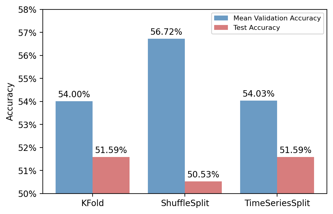
最终的结果显示，Shuffle 方法在验证集上的表现依旧是很不错的，但在测试集上并不总是占优。而时序交叉验证整体表现比较稳健。

在训练时间上，由于控制了训练集样本量，三种方法的训练耗时基本相同。

结论和建议¶

本文比较了 K 折、Shuffle 和时序这三种交叉验证的方法，发现时序交叉验证不会产生数据泄露的问题，在验证集上的准确率虽然不高，但在测试集上的表现更稳健，并且在训练时间开销上也更占优势。
对时序属性较强的数据集，例如金融数据、医疗监测数据、销量数据等等，更推荐使用时序交叉验证的方法调整超参数，避免使用未来信息。
交叉验证的过程就是不断计算、寻找最优参数。这个过程看上去没有什么技术含量，但它本质上是“选择算法的算法”，对模型结果也有不小的影响，所以我们应当引起重视。

K 折、随机和时间序列交叉验证的 Python 实现¶

特征工程代码片段¶

词频统计¶

TF-IDF¶

2-gram TF-IDF¶

交叉验证——以 XGBoost 为例¶

交叉验证的数据¶

定义交叉验证划分方法的实例¶

定义函数，绘制不同交叉验证方法下，训练集和验证集的分布情况¶

绘制不同交叉验证方法下，训练集和验证集的分布情况¶

定义函数，汇总不同交叉验证方法下的最优参数¶

定义函数，绘制不同交叉验证方法下的平均验证集准确率和测试集准确率¶

时序交叉验证的实现方法¶

网格搜索¶

随机搜索¶

交叉验证——对比多种模型¶

控制训练集样本量¶

在相同训练集样本量的情况下，比较各模型的优劣¶

结论和建议¶

评论