使用 AdaBoost 进行回归预测
AdaBoost 是一种自适应提升的树模型,它对预测错误的样本增加权重,以提高预测准确率。
数据集 HousePrices 包含了美国 Iowa 州 Ames 地区住宅的价格,以及这些住宅的相关信息,包括建造时间、房顶材料、车库面积等等,其中该数据集中有 1100 大小的训练数据和 360 大小的测试集。
下面我们通过 AdaBoost 方法,用房子的特征来预测房子的售价。
Python
# 导入包
import pandas as pd
import numpy as np
import matplotlib.pyplot as plt
from matplotlib.ticker import FuncFormatter

plt.rcParams["font.sans-serif"] = ["SimHei"]
plt.rcParams["axes.unicode_minus"] = False
from scipy.stats import pearsonr
from sklearn.preprocessing import MinMaxScaler
from sklearn.feature_selection import VarianceThreshold
from sklearn.feature_extraction import FeatureHasher
from sklearn.tree import DecisionTreeRegressor
from sklearn.ensemble import AdaBoostRegressor
from sklearn import metrics
读取数据
Python
# 读取数据
train = pd.read_excel("HousePrices.xlsx", sheet_name="train", engine="openpyxl")
test = pd.read_excel(
    "HousePrices.xlsx", sheet_name="test", header=None, engine="openpyxl"
)
test.columns = train.columns
x_train = train.drop(["SalePrice"], axis=1)
y_train = train["SalePrice"]
x_test = test.drop(["SalePrice"], axis=1)
y_test = test["SalePrice"]
处理缺失值
查看缺失值
Python
column_with_null = x_train[x_train.columns[x_train.isna().any()]].isnull().sum()
print(column_with_null)
Text Only
## LotFrontage      192
## Alley           1031
## MasVnrType         6
## MasVnrArea         6
## BsmtQual          31
## BsmtCond          31
## BsmtExposure      32
## BsmtFinType1      31
## BsmtFinType2      32
## FireplaceQu      524
## GarageType        61
## GarageYrBlt       61
## GarageFinish      61
## GarageQual        61
## GarageCond        61
## PoolQC          1098
## Fence            892
## MiscFeature     1054
## dtype: int64
适合用均值填充的列:
Python
# 适合用均值填充的列
fillna_with_mean = ["LotFrontage", "MasVnrArea", "GarageYrBlt"]

for col in fillna_with_mean:
    x_train[col].fillna(x_train[col].mean(), inplace=True)
    x_test[col].fillna(x_test[col].mean(), inplace=True)
适合用'None'填充的列:
Python
# 适合用 None 填充的列
fillna_with_none = list(set(x_train.columns) - set(fillna_with_mean))

for col in fillna_with_none:
    x_train[col].fillna("None", inplace=True)
    x_test[col].fillna("None", inplace=True)
特征编码
大部分特征均为文本型,且包含多个无序的文本值。可以将这些文本值通过哈希编码转换为数值型,以便于后续的建模。
使用n_features参数控制哈希编码的维度,这里将维度设为 2,即将文本值转换为二维的数值型特征。数据集中的特征最多有 10 余个唯一值,因此二维哈希值足以对数据集中的特征进行编码。
Python
# 文本特征的列
text_features = list(x_train.columns[x_train.dtypes == "object"])

# # 哈希编码器
for col in text_features:
    hash_encoder = FeatureHasher(n_features=2, input_type="string")
    # 对原始特征进行编码,得到哈希值数组
    x_train_col_hashed = hash_encoder.fit_transform(x_train[col]).toarray()
    x_test_col_hashed = hash_encoder.transform(x_test[col]).toarray()
    # 转换为数据框
    x_train_col_hashed = pd.DataFrame(
        x_train_col_hashed, columns=[col + "_" + str(i) for i in range(1, 2 + 1)]
    )
    x_test_col_hashed = pd.DataFrame(
        x_test_col_hashed, columns=[col + "_" + str(i) for i in range(1, 2 + 1)]
    )
    # 删除原有的文本特征
    x_train.drop(col, axis=1, inplace=True)
    x_test.drop(col, axis=1, inplace=True)
    # 将哈希编码后的特征添加到数据集中
    x_train = pd.concat([x_train, x_train_col_hashed], axis=1)
    x_test = pd.concat([x_test, x_test_col_hashed], axis=1)
特征选择
移除低方差特征
Python
# 删除 id 列
x_train.drop(["Id"], axis=1, inplace=True)
x_test.drop(["Id"], axis=1, inplace=True)
# 将特征进行最小最大归一化
scaler = MinMaxScaler()
x_train = pd.DataFrame(
    scaler.fit_transform(x_train), index=x_train.index, columns=x_train.columns
)
x_test = pd.DataFrame(
    scaler.transform(x_test), index=x_test.index, columns=x_test.columns
)
# 移除低方差(归一化后方差小于 0.005)特征
selector = VarianceThreshold(threshold=0.005)
selector.fit(x_train)
# 打印因为低方差被移除的特征
Text Only
## 因为低方差被移除特征: Index(['LotArea', '3SsnPorch', 'PoolArea', 'MiscVal', 'Street_1', 'Street_2',
##        'Utilities_1', 'Utilities_2', 'Condition2_1', 'Condition2_2',
##        'RoofMatl_1', 'Foundation_2', 'Heating_2', 'CentralAir_1',
##        'CentralAir_2', 'PavedDrive_1', 'PavedDrive_2', 'PoolQC_1', 'PoolQC_2',
##        'MiscFeature_1', 'MiscFeature_2'],
##       dtype='object')
Python
x_train = x_train.loc[:, selector.get_support()]
x_test = x_test.loc[:, selector.get_support()]
移除高相关特征中方差较低的那一个
由于特征变量众多,这里不再绘制相关系数热力图。
Python
corr = x_train.corr()
# 打印相关性绝对值大于 0.8 的特征
corr = corr.abs()
corr = corr.where(np.triu(np.ones(corr.shape), k=1).astype(bool))
corr = corr.stack()
corr = corr[corr > 0.8]
print("相关性绝对值大于 0.8 的特征:", [i for i in corr.index])
# 从数据集中移除相关性绝对值大于 0.8 的特征中方差较小的特征
Text Only
## 相关性绝对值大于0.8的特征: [('TotalBsmtSF', '1stFlrSF'), ('GrLivArea', 'TotRmsAbvGrd'), ('Fireplaces', 'FireplaceQu_1'), ('GarageCars', 'GarageArea'), ('LotShape_1', 'LotShape_2'), ('LandContour_1', 'LandContour_2'), ('LotConfig_1', 'LotConfig_2'), ('RoofStyle_1', 'RoofStyle_2'), ('Exterior1st_1', 'Exterior2nd_1'), ('Exterior1st_2', 'Exterior2nd_2'), ('ExterQual_1', 'ExterQual_2'), ('ExterCond_1', 'ExterCond_2'), ('BsmtQual_1', 'BsmtQual_2'), ('BsmtCond_1', 'BsmtCond_2'), ('HeatingQC_1', 'HeatingQC_2'), ('Electrical_1', 'Electrical_2'), ('KitchenQual_1', 'KitchenQual_2'), ('GarageType_1', 'GarageFinish_1'), ('GarageType_1', 'GarageQual_1'), ('GarageType_1', 'GarageCond_1'), ('GarageType_1', 'GarageCond_2'), ('GarageFinish_1', 'GarageQual_1'), ('GarageFinish_1', 'GarageCond_1'), ('GarageFinish_1', 'GarageCond_2'), ('GarageQual_1', 'GarageQual_2'), ('GarageQual_1', 'GarageCond_1'), ('GarageQual_1', 'GarageCond_2'), ('GarageQual_2', 'GarageCond_1'), ('GarageCond_1', 'GarageCond_2')]
Python
feature_to_remove = []
corr = corr.reset_index()
corr.columns = ["feature1", "feature2", "corr"]
for row in corr.itertuples():
    if x_train[row.feature1].var() < x_train[row.feature2].var():
        feature_to_remove.append(row.feature1)
    else:
        feature_to_remove.append(row.feature2)
feature_to_remove = list(set(feature_to_remove))
print("相关性绝对值大于 0.8 的特征中方差较小的特征:", feature_to_remove)
Text Only
## 相关性绝对值大于0.8的特征中方差较小的特征: ['ExterQual_2', 'BsmtCond_1', 'GrLivArea', 'GarageType_1', 'Exterior1st_1', '1stFlrSF', 'GarageQual_2', 'LotShape_1', 'HeatingQC_1', 'GarageCond_1', 'LandContour_2', 'ExterCond_2', 'RoofStyle_2', 'Electrical_2', 'BsmtQual_1', 'GarageFinish_1', 'KitchenQual_2', 'Fireplaces', 'Exterior2nd_2', 'GarageArea', 'LotConfig_1', 'GarageCond_2']
Python
x_train.drop(feature_to_remove, axis=1, inplace=True)
x_test.drop(feature_to_remove, axis=1, inplace=True)
移除与标签相关性较低的特征
Python
# 移除与标签相关性绝对值小于 0.02 的特征
feature_to_remove = []
for i in x_train.columns:
    pearson_corr = pearsonr(x_train[i], y_train)[0]
    if abs(pearson_corr) < 0.02:
        feature_to_remove.append(i)
print("与标签相关性绝对值小于 0.02 的特征:", feature_to_remove)
Python
x_train.drop(feature_to_remove, axis=1, inplace=True)
x_test.drop(feature_to_remove, axis=1, inplace=True)
最终选择的特征
Text Only
## 最终选择的特征 ['MSSubClass' 'LotFrontage' 'OverallQual' 'OverallCond' 'YearBuilt'
##  'YearRemodAdd' 'MasVnrArea' 'BsmtFinSF1' 'BsmtUnfSF' 'TotalBsmtSF'
##  '2ndFlrSF' 'LowQualFinSF' 'BsmtFullBath' 'BsmtHalfBath' 'FullBath'
##  'HalfBath' 'BedroomAbvGr' 'KitchenAbvGr' 'TotRmsAbvGrd' 'GarageYrBlt'
##  'GarageCars' 'WoodDeckSF' 'OpenPorchSF' 'EnclosedPorch' 'ScreenPorch'
##  'MoSold' 'YrSold' 'MSZoning_1' 'MSZoning_2' 'Alley_1' 'Alley_2'
##  'LotShape_2' 'LotConfig_2' 'LandSlope_1' 'LandSlope_2' 'Neighborhood_1'
##  'Neighborhood_2' 'Condition1_1' 'Condition1_2' 'BldgType_1' 'BldgType_2'
##  'HouseStyle_1' 'HouseStyle_2' 'RoofStyle_1' 'RoofMatl_2' 'Exterior1st_2'
##  'MasVnrType_1' 'MasVnrType_2' 'ExterQual_1' 'ExterCond_1' 'Foundation_1'
##  'BsmtQual_2' 'BsmtCond_2' 'BsmtExposure_1' 'BsmtExposure_2'
##  'BsmtFinType1_1' 'BsmtFinType1_2' 'BsmtFinType2_1' 'BsmtFinType2_2'
##  'Heating_1' 'HeatingQC_2' 'Electrical_1' 'KitchenQual_1' 'Functional_1'
##  'FireplaceQu_1' 'FireplaceQu_2' 'GarageType_2' 'GarageFinish_2'
##  'GarageQual_1' 'Fence_1' 'Fence_2' 'SaleType_1' 'SaleType_2'
##  'SaleCondition_1' 'SaleCondition_2']
构建 AdaBoost 分类器
Python
adaboost_reg = AdaBoostRegressor(
    DecisionTreeRegressor(max_depth=5), n_estimators=100, learning_rate=0.1
)
adaboost_reg.fit(x_train, y_train)
Text Only
## AdaBoostRegressor(base_estimator=DecisionTreeRegressor(max_depth=5),
##                   learning_rate=0.1, n_estimators=100)
模型评价
Python
# 模型评价
def evaluate(y_test, y_pred):
    print("均方误差:", metrics.mean_squared_error(y_test, y_pred))
    print(
        "平均相对误差:{:.2%}".format(metrics.mean_absolute_percentage_error(y_test, y_pred))
    )


evaluate(y_test, y_pred)
参数调优:迭代次数
由于训练耗时较久,在此博文中对 n_estimators 的范围不设得过于密集。
Python
n_estimators_range = range(100, 2001, 300)
mean_squared_error_list = []
mean_absolute_percentage_error_list = []
for n_estimators in n_estimators_range:
    adaboost_reg = AdaBoostRegressor(
        DecisionTreeRegressor(max_depth=5), n_estimators=n_estimators, learning_rate=0.1
    )
    adaboost_reg.fit(x_train, y_train)
    y_pred = adaboost_reg.predict(x_test)
    mean_squared_error_list.append(metrics.mean_squared_error(y_test, y_pred))
    mean_absolute_percentage_error_list.append(
        metrics.mean_absolute_percentage_error(y_test, y_pred)
    )
Text Only
## AdaBoostRegressor(base_estimator=DecisionTreeRegressor(max_depth=5),
##                   learning_rate=0.1, n_estimators=100)
## AdaBoostRegressor(base_estimator=DecisionTreeRegressor(max_depth=5),
##                   learning_rate=0.1, n_estimators=400)
## AdaBoostRegressor(base_estimator=DecisionTreeRegressor(max_depth=5),
##                   learning_rate=0.1, n_estimators=700)
## AdaBoostRegressor(base_estimator=DecisionTreeRegressor(max_depth=5),
##                   learning_rate=0.1, n_estimators=1000)
## AdaBoostRegressor(base_estimator=DecisionTreeRegressor(max_depth=5),
##                   learning_rate=0.1, n_estimators=1300)
## AdaBoostRegressor(base_estimator=DecisionTreeRegressor(max_depth=5),
##                   learning_rate=0.1, n_estimators=1600)
## AdaBoostRegressor(base_estimator=DecisionTreeRegressor(max_depth=5),
##                   learning_rate=0.1, n_estimators=1900)
Python
def to_percent(temp, position):
    return "%1.1f" % (100 * temp) + "%"


# 绘制迭代次数与测试误差的关系图
fig = plt.figure(figsize=(9, 6), dpi=200)
ax1 = fig.add_subplot(111)
ax1.plot(
    n_estimators_range,
    mean_squared_error_list,
    "r-o",
    markerfacecolor="none",
    label="均方误差(左轴)",
)
ax1.set_xlabel("AdaBoost 迭代次数")
ax1.set_ylabel("均方误差")
ax2 = ax1.twinx()
ax2.plot(
    n_estimators_range,
    mean_absolute_percentage_error_list,
    "b-o",
    markerfacecolor="none",
    label="平均相对误差(右轴)",
)
ax2.set_ylabel("平均相对误差", rotation=270, labelpad=15)
# y 轴百分比
ax2.yaxis.set_major_formatter(FuncFormatter(to_percent))
fig.legend(loc=1, bbox_to_anchor=(0.88, 0.85))
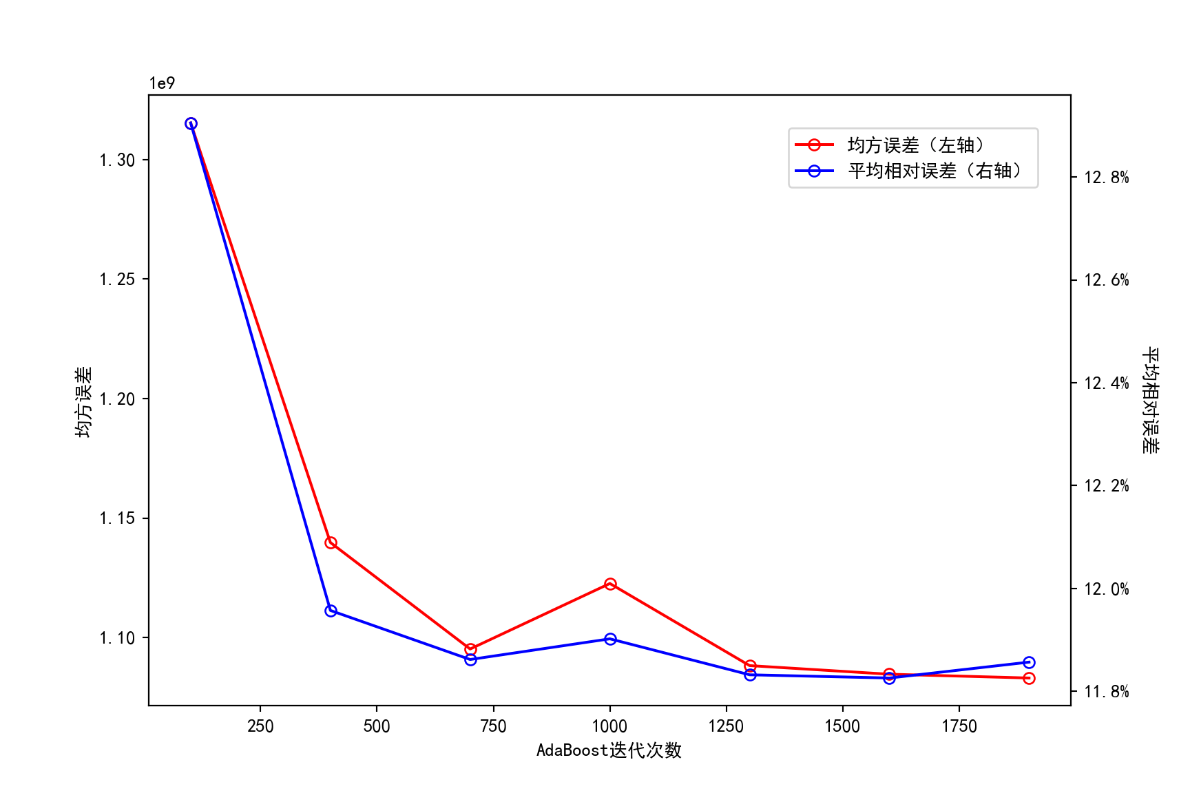
可以看到,当迭代次数增加到 1000 左右时,模型在测试集上的平均相对误差基本稳定在 11.8% 左右。因此,将最好的迭代次数设为 1000。
与决策树做对比
Python
max_depth_range = range(2, 21)
mean_squared_error_list_decision_tree = []
mean_absolute_percentage_error_list_decision_tree = []
for max_depth in max_depth_range:
    decision_tree_reg = DecisionTreeRegressor(max_depth=max_depth)
    decision_tree_reg.fit(x_train, y_train)
    y_pred = decision_tree_reg.predict(x_test)
    mean_squared_error_list_decision_tree.append(
        metrics.mean_squared_error(y_test, y_pred)
    )
    mean_absolute_percentage_error_list_decision_tree.append(
        metrics.mean_absolute_percentage_error(y_test, y_pred)
    )
Text Only
## DecisionTreeRegressor(max_depth=2)
## DecisionTreeRegressor(max_depth=3)
## DecisionTreeRegressor(max_depth=4)
## DecisionTreeRegressor(max_depth=5)
## DecisionTreeRegressor(max_depth=6)
## DecisionTreeRegressor(max_depth=7)
## DecisionTreeRegressor(max_depth=8)
## DecisionTreeRegressor(max_depth=9)
## DecisionTreeRegressor(max_depth=10)
## DecisionTreeRegressor(max_depth=11)
## DecisionTreeRegressor(max_depth=12)
## DecisionTreeRegressor(max_depth=13)
## DecisionTreeRegressor(max_depth=14)
## DecisionTreeRegressor(max_depth=15)
## DecisionTreeRegressor(max_depth=16)
## DecisionTreeRegressor(max_depth=17)
## DecisionTreeRegressor(max_depth=18)
## DecisionTreeRegressor(max_depth=19)
## DecisionTreeRegressor(max_depth=20)
Python
# 绘制决策树最大树深度与测试误差的关系图
fig = plt.figure(figsize=(9, 6), dpi=200)
ax1 = fig.add_subplot(111)
ax1.plot(
    max_depth_range,
    mean_squared_error_list_decision_tree,
    "r-o",
    markerfacecolor="none",
    label="均方误差(左轴)",
)
ax1.set_xticks(max_depth_range)
ax1.set_xlabel("决策树最大树深度")
ax1.set_ylabel("均方误差")
ax2 = ax1.twinx()
ax2.plot(
    max_depth_range,
    mean_absolute_percentage_error_list_decision_tree,
    "b-o",
    markerfacecolor="none",
    label="平均相对误差(右轴)",
)
ax2.set_ylabel("平均相对误差", rotation=270, labelpad=15)
# y 轴百分比
ax2.yaxis.set_major_formatter(FuncFormatter(to_percent))
fig.legend(loc=1, bbox_to_anchor=(0.88, 0.85))
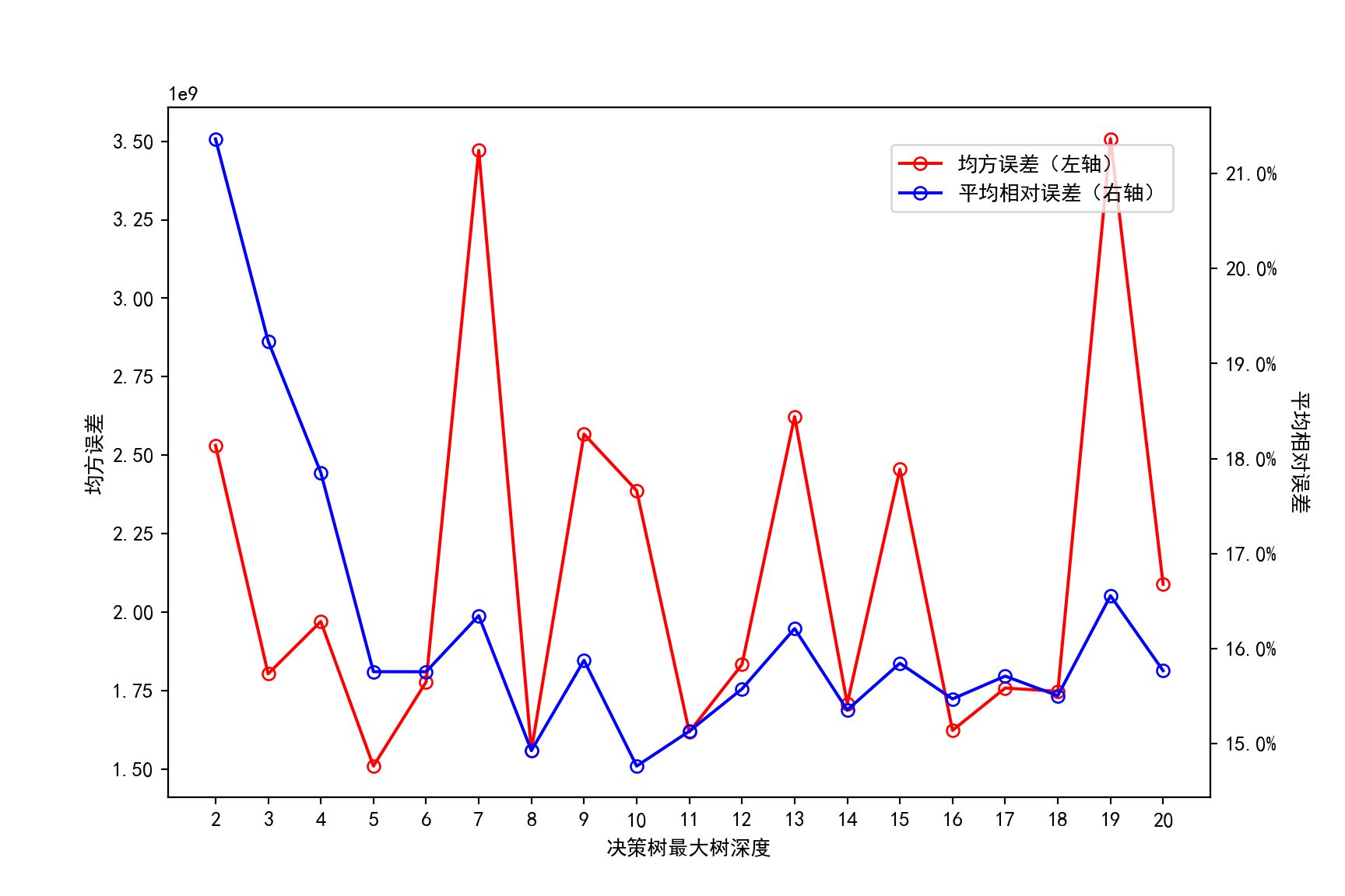
可以看到,决策树中最大数深度大于 5 时,模型开始出现过拟合现象。最优的最大树深度为 5,此时模型在测试集上的平均相对误差约为 15%,高于 AdaBoost 模型的 11.8%。